How to freeze an area in Excel. Translation of "in order to secure" in Chinese

Microsoft Excel has a wide range of different functions. With its help, the user can create tables, analyze data based on the created summary data, build charts and graphs, and calculate values ​​using the necessary formulas and functions. And besides all this, using Excel, you can also view large tables.

If you have a lot of data recorded in rows and columns, all you need to do is capture the columns and rows. Then you can scroll through it and always see, for example, the header.

So, let's figure out how you can freeze the required area in Excel.

First row and column

Let's take the following example, in which the names for all the columns are labeled. Go to the “View” tab and click on the button "To fix areas". From the drop-down menu you can select an item with the appropriate name.

Button "...top line" will allow you to fix the row numbered “1”. As a result, when scrolling through the data, it will always remain visible.

Please note that such rows and columns will be underlined in the table with a black line.

If you select "...first column", then when you scroll the sheet to the right or left, column “A” will always remain in place.

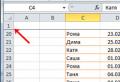
In this case, this is not suitable, since the first column is located under the letter “C”, and the required line is numbered “3”.

Required row

In order to attach a header to an Excel table, which is located in an arbitrary place on the sheet, we will do the following. We select the row that is located immediately under the header, in our case it is 4. You can read a detailed article about selection methods. Now click on the button "To fix areas" and select the item of the same name from the drop-down menu.

As you can see, when scrolling through the table, the pinned header remains in place.

Required column

In order to fix the first column for the entered data, which is not in A, select the adjacent one - in the example it is D. Now click on the button "To fix areas".

You can make sure that when you swipe to the right, C stays in place.

Fast way

To anchor the first column and row in a table, select the cell that is immediately below their intersection: in the example, D4. Then click on the button we are already familiar with. Horizontal lines will appear to indicate the locked area.

How to delete

If you need to delete a frozen area in Excel, click the button "To fix areas". In the drop-down list you will see that now at the very top there is “Unlock…”, click on it.

As you can see, freezing the desired area in Excel is quite simple. Using these recommendations, you can fix the table header, its first row or column.

Microsoft programs are popular because they are convenient both for working with office documents and for personal purposes. Excel is a program that has a large number of different functions that allows you to work with large and massive tables, even on weak computers. In order to understand all the functionality, you need to spend a lot of time, so next we will talk about how it is possible to attach a header in Excel.

How to attach a header in Excel

This can be done either with the help of a special tool that will allow you to print it on each page, or with the help of another that allows you to secure the top line, and when scrolling, the line will be displayed constantly at the top. You can attach the leftmost column in the same way. How can this be done?

In Excel 2003/2007/2010

To attach a header in Excel 2003, 2007 or 2010, you need to follow a few simple steps:

In Excel 2013/2016

In Excel 2016, everything is done in a fairly similar way. Here are step-by-step instructions for pinning in the new Excel:

With this pinning, a row or column will always be visible, which is quite convenient when working with large tables, since scrolling them down in standard mode hides the header.

How do I attach a header to each page for printing?

In the case when you need to print such a line on each page, you need to do the following:

After these operations, when printing, the header will be displayed on each of the printed sheets; you can print the entire table.

Based on this, making pins in Excel is actually quite simple, for which you just need to remember the sequence and what operations need to be performed, and then working in Microsoft Excel will bring you nothing but pleasure.

Video: How to attach a header in Excel?

For some purposes, users want the table header to be visible at all times, even when the sheet scrolls far down. In addition, quite often it is required that when printing a document on physical media (paper), a table header is displayed on each printed page. Let's find out in what ways you can pin a title in Microsoft Excel.

If the table header is located on the top line, and itself occupies no more than one line, then freezing it is a simple operation. If there are one or more blank lines above the title, they will need to be removed in order to use this pinning option.

In order to freeze the title, while in the “View” tab of Excel, click on the “Freeze Areas” button. This button is located on the ribbon in the Window tool group. Next, in the list that opens, select the “Lock top row” option.

After this, the title located on the top line will be fixed, constantly being within the boundaries of the screen.

Freeze an area

If for some reason the user does not want to delete the existing cells above the header, or if it consists of more than one line, then the above pinning method will not work. You will have to use the option of pinning the area, which, however, is not much more complicated than the first method.

First of all, move to the “View” tab. After that, click on the leftmost cell located under the heading. Next, click on the “Pin Areas” button, which was already mentioned above. Then, in the updated menu, again select the item with the same name - “Pin areas”.

After these actions, the table title will be fixed on the current sheet.

Unpin a title

Regardless of which of the two listed methods the table header is pinned, in order to unpin it, there is only one way. Again, click on the button on the “Lock Areas” ribbon, but this time select the “Unlock Areas” option that appears.

Following this, the pinned header will become unpinned, and when you scroll down the sheet, it will no longer be visible.

Freeze the header when printing

There are times when printing a document requires that a header be present on every page printed. Of course, you can manually “break” the table and enter the heading in the right places. But, this process can take a significant amount of time, and, in addition, such a change can destroy the integrity of the table and the order of calculations. There is a much easier and safer way to print a table with a heading on each page.

First of all, move to the “Page Layout” tab. We are looking for the “Sheet Options” settings block. In its lower left corner there is an icon in the form of an inclined arrow. Click on this icon.

A window with page parameters opens. Move to the “Sheet” tab. In the field next to the inscription “Print continuous lines on each page” you need to indicate the coordinates of the line on which the heading is located. Naturally, this is not so simple for an untrained user. Therefore, click on the button located to the right of the data entry field.

The window with page parameters is minimized. In this case, the sheet on which the table is located becomes active. We simply select the line (or several lines) on which the title is located. As you can see, the coordinates are entered in a special window. Click on the button located to the right of this window.

The page settings window opens again. All we have to do is click on the “OK” button located in its lower right corner.

All the necessary actions have been completed, but visually you will not see any changes. In order to check whether the table name will now actually be printed on each sheet, move to the “File” tab of the Excel application. Next, go to the “Print” subsection.

On the right side of the window that opens there is a preview area of ​​the printed document. Scroll it down and make sure that when printed, a fixed header will be displayed on each page of the document.

As you can see, there are three ways to assign a title to a Microsoft Excel table. Two of them are intended to be fixed in the spreadsheet editor itself, when working with a document. The third method is used to display a title on each page of the printed document. It is important to remember that you can fix a title by pinning a line only if it is located on one, and the topmost line of the sheet. Otherwise, you need to use the method of pinning areas.

The social network VKontakte is actively developing, providing users with new functionality. As new options appear, they become increasingly difficult to understand, and obvious functions are hidden from users' view. One of these functions is the ability to mount the post on the wall. For a long time now, you can attach a post not only to a group’s page, but also to your personal one. We suggest you figure out how to pin a post on your VKontakte wall in just a few clicks.

The wall of an active social network user is regularly updated with new entries, and useful, interesting or important posts are lowered down in the feed. Scrolling to them is not always convenient, especially when it comes to a musical composition or a photograph that you want to have quick access to. By pinning a post on your personal VKontakte wall, you can be sure that friends, subscribers and simply guests of your page will see it. Since you cannot set a picture or audio recording to your status, it is convenient to use your wall so that the largest number of people can get acquainted with the audio, video or visual post you like.

By following simple steps, you can pin a post on your VKontakte wall:

After completing the steps described above, the selected post will be pinned to the top of your page on the social network. It will remain there until you decide to delete or unpin it.

To unpin a post from your personal VKontakte page you need to:

As you can see, pinning and unpinning a post from a VKontakte wall is very simple, and this procedure takes a few seconds if you know which buttons to press.

How to pin a post on the wall of a VKontakte group?

The system for pinning a post on a public VKontakte page and in a group is no different. It is useful to pin a post when necessary:

• Show new visitors to the community key information about the group’s operating principles or rules;
• To ensure that the maximum number of group visitors gets acquainted with an interesting publication;
• To attract the attention of group visitors to a promotion or sale, if the group is an online store;
• For advertising purposes.

You can pin a post in a VKontakte group by following these steps:

Attention: Only the group administrator can pin a post to a group. Users who do not have the necessary rights will not see the “Pin” button when they click on a post date.

It is important to note that a pinned post in a group or on a public page on VKontakte is not displayed in the general feed, but above – directly below the name of the group and its status.

When working with tables in Excel, it is often necessary to separate the top row or left column from the rest of the table. In this material we will talk about how to freeze an area in Excel using the “Freeze Areas” function.

The “Freeze Area” function allows you to freeze a part of an Excel sheet so that it is always in front of the user’s eyes when scrolling the page. In addition, when sorting data, cells in the pinned area do not participate in the sorting and do not change their location.

In order to freeze an area in Excel, you need to go to the “View” tab and use the “Freeze Areas” button.

When you click on this button, a drop-down menu appears with the following items: freeze areas (this drop-down menu item allows you to freeze an arbitrary part of the Excel sheet), freeze the top row (this drop-down menu item allows you to freeze only one top row), freeze the first column (this drop-down menu item allows you to freeze only the first column). Let's look at all these menu items in order.

The first item “Freeze areas” allows you to freeze any number of first rows and columns. In order to use this function, you need to select a cell that will be located at the intersection of fixed rows and columns.

For example, if you want to freeze the first two columns and the first two rows in an Excel sheet, then you need to select the cell that is in the third column and third row. In other words, you need to select cell C3. After you have selected the desired cell, you need to click on the “Freeze Areas” button and select the first item in the drop-down menu.

After this, vertical and horizontal lines will appear on the Excel sheet, which separate the pinned area from the rest of the sheet.

If you just need to freeze the first column or first row, you can use the Freeze Top Row or Freeze First Column functions. You even have to select cells to use these functions. All you need to do is go to the “View” tab, click on the “Freeze Areas” button and select the appropriate item from the drop-down menu.