home » Adviсe » Building graphs in excel presentation. Theme of the lesson: "MS Excel: Construction of charts and graphs". Building and editing function graphs

Building graphs in excel presentation. Theme of the lesson: "MS Excel: Construction of charts and graphs". Building and editing function graphs

And then copy it into your presentation. This method is also optimal if the data changes regularly and you want the chart to always be up to date. In this case, when copying the chart, keep its link to the original Excel file.

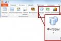
Insert press the button Diagram

Advice: When you insert a chart, small buttons appear near the top right corner of the chart. Use button Chart elements to show, hide, or format items such as axis titles or data labels. Use button Chart styles to quickly change the color or style of a chart. With button Chart Filters you can show or hide the data in the chart.

To create a simple chart from scratch in PowerPoint, on the Insert press the button Diagram, and then select the desired chart.

You can modify a chart in PowerPoint by customizing its appearance, size, and position. Click the chart and then make changes on the tab Constructor, Layout or Format under the green tab Working with charts. To add animation effects, use the tools on the tab Animation.

Note: If the group Working with charts is not displayed, click anywhere in the diagram.

You can change the chart data in PowerPoint. Click the chart and then under the green tab Working with charts select tab Constructor and press the button To change the data. See the article for more information.

Insert a chart or graph into a presentation

To create a simple chart from scratch in PowerPoint, on the Insert press the button Diagram, and then select the desired chart.

Note: To change data in an inserted chart, use the command To change the data. Additional information about the team To change the data see Change data in an existing chart.

Insert an Excel chart or graph into a presentation and link it to data in Excel

Create a chart or graph in Office Excel 2007 and copy and paste it into your PowerPoint 2007 presentation. If the data in the linked Office Excel 2007 file has been updated, you can refresh the chart in PowerPoint using the command Update the data.

For more information about inserting Excel charts and graphs into a PowerPoint presentation, see Copy an Excel chart to another Office program.

Note: If you want to automatically update data in a chart or graph, save the Excel file before inserting the chart or graph.

In Excel, select a chart by clicking on its border and then on the tab home in Group Clipboard click Cut.

In PowerPoint 2007, click the placeholder on the slide or notes page where you want to place the chart.

On the tab home in Group Clipboard click the arrow below the button Insert and select command Insert.

Insert an Excel chart or graph into a presentation and create a data link in an Office Excel 2007 file. When you copy a chart from a saved Office Excel 2007 file and paste it into a presentation, the chart data is linked to that Excel file. If you want to change the data in a chart, you must make changes to the linked worksheet in Office Excel 2007 and then update the data in your PowerPoint presentation. The Excel sheet is a separate file and is not saved with the PowerPoint file.

Note: When you open a presentation that was created in an earlier version of PowerPoint and has a graph or chart created with the Microsoft Graph application, PowerPoint 2007 retains the same appearance and allows you to continue editing the graph or chart.

Figure 2. PowerPoint chart created from sample data in an Excel worksheet

Methodical development

computer science teachers

GBOU school number 638

Alexandrova

Svetlana Nikolaevna

Building charts and graphs

Content:

Why build diagrams?
Chart basis
Basic chart elements
Chart types
Diagramming
Building a pie chart
Building a histogram
Plotting functions
Exercise
Literature

Why build charts?

visual presentation of information
showing ratios of values or trends in tabular data

This is needed for:

Chart Base A table is used as the basis for creating a chart. The rectangular table structure allows us to build a chart based on a rectangular coordinate system. Data elements (individual numbers) plotted on the chart are combined into data series ( a group of consecutive cells located in a row or column of a table).

A diagram is a composite object consisting of the following main elements:

Chart drawing area with grid lines

Y-axis label

coordinate axis

X axis label

header

Data Signatures

Legend - notation

Basic chart elements

Types of charts 1. Pie charts (they are used when the values of a series of data describe the distribution of a certain value or contribute to a single whole).

There are several types of charts. They differ in appearance, purpose, and the number of valid data rows. Here are some of them:

2. Bar or column charts - histograms (this form is convenient for comparing values; several data series can be displayed on one chart).

3. Graphs (they serve to display the dependence of the function value on its argument; time, distance, and other variable can be used as an argument).

Types of charts Any chart is one of the three main categories presented above. There are different options for their design. With volumetric design, data elements are represented by images of three-dimensional figures (parallelepipeds, cylinders, cones, pyramids) to increase visibility.

It's cylindrical

diagram

It's voluminous

pyramid chart

Chart construction

When choosing the type of graphical representation of data (graph, histogram, chart of one kind or another), be guided by what kind of information you need to display. If you want to identify the change in any parameter over time or the relationship between two quantities, you should build a graph. To display shares or percentages, it is customary to use a pie chart. Comparative analysis of data is conveniently presented in the form of a histogram or bar chart.

Chart construction Procedure:

Select the cells containing the data to plot the chart.
In the Charts group on the Insert tab, do one of the following:

Select the chart type and then the chart subtype you want to use.
On the Design tab, in the Location group, click Move Chart.

Building a Chart 4. Click on a chart to open the Chart Tools panel, which contains additional tabs Design, Layout, and Format. With which you can choose a ready-made layout and style for the chart. 5. Format the chart.

Building a pie chart

A table is given that reflects the family's expenses for 4 months. We are interested in what percentage of the family's home budget for this period (build a pie chart).

Look

construction

Building a histogram

A certain company selling ice cream in city K kept records of revenue (in million rubles) for four districts of the city in the summer months of 2000. Construct a histogram of revenue by districts for the summer.

Look

construction

Plotting functions

y1 = 2sinx - 0.5

Look

construction

Task Given a table of forecasting the growth of the population of the Earth. We are interested in the percentage distribution of the population by continent in 2000. Build a chart (pie, volumetric).

Click here and

complete the task!

Forecast of the growth of the population of the Earth (thousand people)
Continent




Australia

Now click on the "Answer" button and check if you completed the task correctly!

Literature

Lavrenov S.M. Excel: Collection of examples and tasks. – M.: Finance and statistics, 2007.
Shafrin Yu.A. Workshop on computer technology, M: ABF, 1997.
Stolyarov A.M. Excel for myself. – M.: DMK Press, 2008.

“Man, undoubtedly, was created to think: this is his main dignity and the main business of life ...”

Blaise Pascal

TOPIC OF THE LESSON:

BUILDING DIAGRAM

PIE CHARTS

GRAPHING

Graphs are used to display the dependence of the values of one value (function) on another (argument); graphs allow you to track the dynamics of data changes.

World population

Graph of the function y=x^2

Example of a graph in spreadsheets

PIE CHARTS

Pie charts are used to display the values (sizes) of parts of a whole; in them, each part of the whole is represented as a sector of a circle, the angular size of which is directly proportional to the size (size) of the part.

The structure of farmland in Russia

Profit from the sale of ice cream

An example of a pie chart in spreadsheets

Histograms (bar charts) are used to compare several values; they display values in vertical or horizontal columns. The heights (lengths) of the columns correspond to the displayed values of the quantities.

Area of the largest states of the world, million km 2

Bar Chart Example

STRUCTURE OF THE DIAGRAM

Data series is the set of values to be displayed on the chart.

Charts allow you to visually compare the values of one or more data series.

Sets of values corresponding to each other from different series are called categories .

Diagrams are built in a rectangular coordinate system, where along the axis X category names are signed, and along the axis Y the values of the data series are marked.

header

Data images

and their names

BUILDING DIAGRAM

In spreadsheets, charts are built under the control of the Chart Wizard, which includes the following main steps:

1) Choice of chart type

2) Selecting the data on which the chart is based

3) Setting up chart design elements

4) Chart placement

Charts in spreadsheets retain their dependence on the data they are based on: when the data changes, the corresponding changes occur in the chart automatically.

ALGORITHM FOR BUILDING DIAGRAM:

Enter data into the table.
Select the required data range.
Go to tab Insert | Diagrams and choose a chart type.

4. Using toolbars "Constructor", "Layout", "Format" format chart elements. Fill in the chart parameters (title, category axes, data axes, data labels, etc.).

5. Select the location of the diagram (on a separate sheet or an existing one).

HOMEWORK

PARAGRAPH 3.3.2

RT No. 125, 126, 127

REFLECTION

TODAY IN THE LESSON I LEARNED…..
I LEARNED….
A LESSON GIVED ME FOR LIFE…..
I WILL DEFINITELY TRY…..
THE LESSON I LIKE THE MOST…
I AM STILL DIFFICULT…
IN THE LESSON I WORKED ... ..
MY MOOD:

Diagram. - Select the type of chart you need in the Standard tab (in our case, Graph). - Click Next. Selecting a Chart Type "title="2) will appear. The easiest way to create a chart is to use the appropriate wizard: - Choose Insert > Chart. - Select the type of chart you need in the Standard tab (in our case, Graph). - Click Next. Chart Type Selection Appears" class="link_thumb"> 3 !} 2) To create a chart, the easiest way is to use the appropriate wizard: - Execute the command Insert > Chart. - Select the type of chart you need in the Standard tab (in our case, Graph). - Click Next. Select Chart Type The following dialog box will appear Diagram. - Select the type of chart you need in the Standard tab (in our case, Graph). - Click Next. Select Chart Type "> Chart" will appear. - Select the desired chart type in the Standard tab (in our case Graph). - Click Next. Select Chart Type The following dialog box "> Chart" will appear. - Select the type of chart you need in the Standard tab (in our case, Graph). - Click Next. Selecting a Chart Type "title="2) will appear. The easiest way to create a chart is to use the appropriate wizard: - Choose Insert > Chart. - Select the type of chart you need in the Standard tab (in our case, Graph). - Click Next. Chart Type Selection Appears"> title="2) To create a chart, the easiest way is to use the appropriate wizard: - Execute the command Insert > Chart. - Select the type of chart you need in the Standard tab (in our case, Graph). - Click Next. Chart Type Selection Appears"> !}

The second dialog box of the wizard allows you to select or edit the data source. Because a range of data was already selected in the worksheet when you started the wizard, it is automatically selected as the data source. The raw numeric data for the chart should be highlighted along with the row and column of table titles so that the appropriate titles automatically appear in the legend and category axis of the chart. Specifying the Data Source Click the Next button to go to the Chart Options dialog box.

Setting the chart parameters 4) In the Chart Name field, enter text - Blood sugar level X-axis (categories) text - date Y-axis (values) text - sugar level Then click on the Next button to go to the fourth window of the wizard, which determines the location of the future chart .

Back forward

Attention! The slide preview is for informational purposes only and may not represent the full extent of the presentation. If you are interested in this work, please download the full version.

Lesson objectives:

Educational:
- learning techniques for constructing and editing various types of charts and graphics;
- consolidation of knowledge when working with various types of spreadsheet data;
- formation of skills for independent work with educational, popular science literature and Internet materials.
Educational:
- development of students' creative thinking, cognitive interest;
- formation of communication skills;
- formation of skills for independent use of computers as a tool for cognitive activity;
- development of independence in the acquisition of knowledge, mutual assistance, speech.
Educational:
- fostering a culture of communication, the ability to work in a group, the ability to listen,
- fostering a caring attitude towards computers and their workplace;
- fostering an objective attitude to the results of work - criticality, the ability to adequately assess the situation.

Lesson type: combined lesson - explanation of new material and consolidation of acquired knowledge.

Type of lesson: practical work.

Equipment:

Student computers
Multimedia projector, screen
Presentation prepared in PowerPoint
Cards with tasks for practical work
Text task

Lesson plan

Organizing time
Announcement of the topic of the lesson and the purpose of the lesson
Expert speech
Presentation of educational material
Practical work on the computer
Expression of expert opinion.
Execution of a test task
Summarizing. Homework Reflection

Material support for the lesson:

IBM PC AT Pentium - one for each student;
OS MS Windows 2003/XP, MS Excel

Literature:

Semakin I. G., Henner E. K. Computer science. Grade 11. M.: BINOM. Knowledge Laboratory, 2002, pp. 96–122.
Informatics and information technologies. Ugrinovich N.D. Textbook for grades 10-11. - M .: Basic Knowledge Laboratory, 2000
Journal “Computer Science and Education” №4 – 2010

What science has your mind not comprehended,
Do not know peace in learning for a moment

Ferdowsi, Persian poet

DURING THE CLASSES

1. Learning new material

In any field of activity, there are many tasks in which the initial data and results must be presented in graphical form. The ability to visualize information in the form of graphs and diagrams is an integral part of modern education. When solving various problems, preparing reports on various disciplines, performing creative tasks, it often becomes necessary to graphically represent numerical data. The main advantage of such a representation is visibility.

- Today in the lesson 5 experts will help to consider this topic. (Experts are prepared in advance by a teacher from among the successful students)

List of issues under study

Diagrams (concept, purpose). Chart objects. Chart types.
Create diagrams Automatically create diagrams (in one step).
Diagram Wizard.
Editing diagrams.
Editing the finished diagram.
Editing individual chart elements.

Diagrams (concept, purpose). Chart Objects

When solving various problems, preparing reports, there is often a need for a graphical representation of numerical data. The main advantage of such a representation is visibility.

Microsoft Excel has the ability to graphically represent data in the form of a chart. Charts are linked to the sheet data they were created from and change each time the sheet data changes. A chart is an insertable object embedded on one of the sheets in a workbook.

Diagram- an object of a spreadsheet that clearly shows the ratio of any values.
Purpose of the chart: Graphical display of data for analysis and comparison.
Chart objects:
chart area- the area in which all the elements of the diagram are located;
plot area- the location of the axes, data series, etc.;
legend- a sample data format;
header- serves to explain the data presented in the diagram;
data labels (markers)– symbols (bars, dots, sectors, etc.) in the diagram representing a single data element;
data series– groups of related data elements in the diagram, the source of which is a single row or a single column of a data table;
axis- a line that bounds one of the sides of the chart construction area and creates a scale for measuring and comparing data on the chart (for a two-dimensional graphic arts– X-axis, Y-axis; for a 3D graph, Z is the vertical axis, and the X and Y axes are located at different angles):
categories– category names correspond to labels along the X axis;
row names– usually correspond to inscriptions along the Y axis;
tick marks- these are short segments that intersect the coordinate axes like marking a ruler.

Chart types.

In MS Excel, you can choose from several types of charts, and each type has several varieties (kinds). The right choice of chart type makes it possible to present the data in the most advantageous way. MS Excel allows you to choose from 14 basic (standard) chart types and 20 additional (non-standard) chart types. Within each of the main chart types, a specific subtype can be selected.
Consider the main ones

bar chart displays the values of different categories, allows you to show multiple data series

Ruled also displays values for different categories, differs in the orientation of the Ox and Oy axes

Schedule presented as data points connected by a thin line, allows you to follow the changes in the proposed data, show several data series

Pie and donut chart only one data series can be shown. The choice of this type is determined by considerations of expediency and visibility

Area Chart displays the change in the values of the series over time, as well as the change in the contribution of individual values.

Three-dimensional (volumetric) diagram refer Histogram, Bar chart, 3D chart, 3D pie chart, Surface

2. Practical work on the computer

Setting Open the MS EXCEL program, display the "Charts" toolbar (Toolbar View - Chart)
Save the workbook under your last name in the "my documents" folder

TASK 1. Building a histogram according to a given table of values

Work technology

1. Rename Sheet1 to "Internet". Build a table according to the model in Fig. 1

2. Find the maximum and minimum share of users by interest in the range C5:C12 using the Function Wizard and Functions MAX, MIN.

3. Select the data range to plot the histogram: B5:C12.

4. Call the Chart Wizard: select the menu command Insert, Chart or click on the Chart Wizard icon and follow its instructions:

Step 1. Choosing a chart type: bar chart> select chart type - histogram
select the type of histogram - a regular histogram, click the Next > button.

Step 2. Select the source data for the chart: since you have already selected the data in step 3 (range B5:C12), click on the Next > button

Step 3. Select Chart Options: On the Titles tab, enter text in the Chart Name - Internet User Interests, X (Category) Axis - Interest Type, Y (Values) Axis - User Percentage; click Next > .

5. Position the chart area in the range A16:D40 (to move the selected chart area, use the Drag-and-Drop method, to resize the frame, work with the chart frame handles

6. Save the changes to the file.

7. Compare your result with Fig. 2. Present the results of the work to the expert.

TASK 2. Editing histogram objects

Edit the histogram according to fig. 2.

Work technology.

1. Select the specified diagram object (by double-clicking the left mouse button), select the appropriate tab, make the following changes to the object's parameters, and click the OK button.

Chart object parameters:

The font of the title, legend, axis names (brand, quantity) is Arial, size is 8.
Chart area format: fill method - gradient, colors - two colors, hatching type - diagonal 1.
Chart area format: texture in fill methods - parchment.
Category axis and value axis format: line color - green, line thickness

2. Plot the Gridlines of the X and Y Axes
select menu command Chart, Chart Options, tab grid lines;
in sections X axis (categories) And Y-axis (values) select main lines.

3. Set the format of the grid lines of the X and Y axes: line type - dotted, color - dark turquoise.

4. Save changes to file

TASK 3. Construction of graphs of functions.

Plot the following functions

Y1(x) = x 2 - 1
Y2(x) = x 2 + 1
Y3(x) = 10 * Y1(x)/Y2(x)
The range of the argument is [–2;2] with a step of 0.2..

Work technology: table preparation

1. Go to Sheet2, rename Sheet2 to "Charts":
right-click on the label Sheet2 - call the context menu;
select Rename.

2. Prepare a table on the “Graphics” sheet according to Figure 3: enter the names of the columns in cells A1:D1; in the future, the names of the functions Yl(x), Y2(x), Y3(x) will form the text of the legend;
fill in the argument column (x) from -2 to 2 in increments of 0.2. To do this, use any method known to you to autocomplete the range.

3. Fill in the columns of functions, i.e. enter in columns B, C, D the values of the functions at the corresponding points. To do this, enter independently in cells B2, C2, D2 formulas, the mathematical notation of which, Yl(x) = x2 - 1, Y2(x) = x2 + 1, Y3(x) = 10*Yl(x)/Y2(x)

4. Copy the formulas to the rest of the table cells (use the fill handle).

5. Design the resulting table and save the changes in the file. Present the results of your work

4. Building and editing function graphs

1. Highlight the data range for plotting A1:D22.

2. Build graphs using Chart Wizard: chart type - scatter, type - scatter plot with values connected by smooth lines without markers.

3. Edit the graphs according to fig. 4 and save the changes to the file. Present the results of your work.

Then open the tasks for independent work. Complete the table below, enter the necessary data, set the required data formats. Plot the charts ( Annex 1 )

5. Expressing the opinion of experts on the work

6. Performing a test task

7. Summing up

8. Homework: Glushakov V.F., Melnikov V.E., “Fundamentals of Informatics”, pp. 256-258, answer to counter. questions

Type