Excel is the number of cells with a specific value. Count if function: count the number of cells by a specific criterion in excel. Using VBA functions
Good afternoon, dear reader!
I want to devote this article to the repetitions of those values \u200b\u200bthat occur in your table, that is, we will learn how to count repetitions in Excel. This feature will be useful when calculating the same values \u200b\u200bin the required range, it will help when you need a lot, for example, how many employees made checks, how many times they worked with this or that supplier, and much more.
First, let's look at how the columns with data look, the repetitions in which, we will actually count. For example, let's take a list of employees who make sales.  Now you can count how many times an employee has made sales, that is, we simply count how many repetitions of his name in a column. This can be done in several ways:
Using the COUNTIF function
In Excel, it is extremely easy to make such a calculation, just use it and it will do everything for you in a few seconds. In our case, the formula will look like this:
\u003d COUNTIF ($ B $ 2: $ B $ 11; B15)  In the first argument "range" $ B $ 2: $ B $ 11, we indicate the one in which the duplicate data will be counted. Important! It is not allowed to specify a random data range. Its peculiarity is that it can only be a range of cells or a reference to a specific cell.
The second argument "criterion" we put an indication on the cell by which the calculation of similar data will be made. If he alone, you can register it manually as a text word and specify “Nagaev A.V.” instead of the cell address “B15”, the result will be the same, but only in one specific case, the possibility of automating the table will be significantly reduced.
Additional Information! In addition to directly specifying data retrieval, the COUNTIF function can work with wildcards. There are two types of such signs "?" and "*", they can be used only when working with symbols. The "*" sign allows you to replace absolutely any number of values, and the "?" replaces only one character.
To work with numeric values, you must use the comparison operator signs: "\u003e", "<», «<>"And" \u003d ". For example, to count numerical values \u200b\u200bgreater than "zero", write "\u003e 0", and to count non-empty cells, you need to specify "<>».
Using the COUNTIFS function
When you need to count repetitions in Excel, but already according to several criteria, then you need to work with the COUNTIFS function, which can easily and easily do this.
In my example, I will add a sales category by city and use the formulas to collect the repetitions I need:
\u003d COUNTIFS ($ B $ 2: $ B $ 11; B14; $ C $ 2: $ C $ 11; C14)  Note that the spelling of the function is absolutely similar to the previous COUNTIF function, the difference is only in their number. In our example, there are two of them, but the function can work with 127 ranges as well.
We work with the DLSTR function
Now let's consider a situation when not everything is so simple and orderly, when information is knocked down in one cell, for example, "Nagaev Gavrosh Karopachev Kozubenko Nagaev Gavrosh Kozubenko Nagaev Nagaev"... In this case, statistical functions will not help us, we need to count the symbols and check the repetitions of the values \u200b\u200bwith the specified standard. For these purposes, there are many other useful functions, using which this can be done quite simply:
\u003d (DLSTR ($ B $ 2) -LSTR (SUBSTITUTE ($ B $ 2; B5; ""))) / DLSTR (B5)  So, using, we calculate how many characters are contained in the cell "$ B $ 2" and "B5", the result will be "71". And then with the help we replace the current value with "empty", we get the result "47". The next step is to subtract our remainder "71-47 \u003d 24" from the total number of characters and divide by the number of characters in one value "24/6 \u003d 4", as a result we get how many times in a line, the required result is found ... Answer: 4. (This result considering only the first search string).
With VBA functions
The last option considered is to count the number of repetitions using a function created in VBA. I did not write the functions, but simply offer you the previously found option to simplify your work.
First you need to start VBA and insert a new module using the commands "Insert" - "Module".  In the created module window, you paste the function code:
Function GetRepeat (sTxt As String, sCntWord As String) GetRepeat \u003d (Len (sTxt) - Len (Replace (sTxt, sCntWord, ""))) / Len (sCntWord) End Function
Function GetRepeat (sTxt As String, sCntWord As String) GetRepeat \u003d (Len (sTxt) - Len (Replace (sTxt, sCntWord, ""))) / Len (sCntWord) End Function |
After all this, call "Function Manager" in the control panel or using Ctrl + F3 and in the category "User-defined" you have a new required function.  We use the function on the cell in a standard way using the formula:
\u003d GetRepeat ($ B $ 2; B8)where:

And that's all for me! I was very happy to help and share information about the ability to count repetitions in Excel. If you have something to supplement the article, write it in the comments. I am waiting for your likes, this is the best incentive to see the benefits of my articles!
Our every day is a bank account, and money on it is our time. There are no rich and poor here, everyone has 24 hours.
Christopher Rice
In some cases, the user is asked not to count the sum of the values \u200b\u200bin a column, but to count their number. That is, simply put, you need to count how many cells in a given column are filled with certain numeric or text data. In Excel, there are a number of tools that can solve this problem. Let's consider each of them separately.
Depending on the user's goals, Excel can count all the values \u200b\u200bin a column, only numerical data and those that meet a certain specified condition. Let's look at how to solve the assigned tasks in different ways.
Method 1: indicator in the status bar
This method is the simplest and requires the least amount of steps. It allows you to count the number of cells containing numeric and text data. You can do this simply by looking at the indicator in the status bar.
To complete this task, just hold down left button mouse and select the entire column in which you want to count the values. As soon as the selection is made, in the status bar, which is located at the bottom of the window, near the parameter "Number" the number of values \u200b\u200bcontained in the column will be displayed. Cells filled with any data (numeric, text, date, etc.) will participate in the calculation. Empty items will be ignored when counting.

In some cases, the number of values \u200b\u200bindicator may not appear in the status bar. This means that it is most likely disabled. To enable it, click right click mouse on the status bar. A menu appears. In it you need to check the box next to the item "Number"... After that, the number of cells filled with data will be displayed in the status bar.

The disadvantages of this method include the fact that the result obtained is not recorded anywhere. That is, as soon as you deselect it, it disappears. Therefore, if it is necessary to fix it, you will have to record the resulting total manually. In addition, using this method, you can count only all the cells filled with values \u200b\u200band you cannot set the counting conditions.
Method 2: COUNT operator
Using the operator COUNTas in the previous case, it is possible to count all the values \u200b\u200blocated in the column. But unlike the option with an indicator in the status bar, this method provides an opportunity to fix the result in a separate element sheet.
The main task of the function COUNT, which belongs to the statistical category of operators, is just counting the number of nonblank cells. Therefore, we can easily adapt it to our needs, namely, to count the elements of a column filled with data. The syntax for this function is as follows:
COUNT (value1; value2; ...)
In total, the operator can have up to 255 general group arguments "Value"... The arguments are just references to cells or a range in which you want to count values.


As you can see, unlike the previous method, this option offers to output the result to a specific sheet element with its possible saving there. But unfortunately the function COUNT all the same does not allow specifying the selection conditions for values.
Method 3: COUNT operator
Using the operator SCORE only numerical values \u200b\u200bin the selected column can be counted. It ignores text values \u200b\u200band does not include them in the grand total. This function also belongs to the category of statistical operators, like the previous one. Its task is to count cells in the selected range, and in our case, in a column that contains numeric values. The syntax for this function is almost identical to the previous statement:
COUNT (value1; value2; ...)
As you can see, the arguments for SCORE and COUNT are exactly the same and are cell or range references. The difference in syntax is only in the name of the operator itself.


Method 4: the COUNTIF operator
Unlike the previous methods, using the operator COUNTIF allows you to set conditions corresponding to the values \u200b\u200bthat will take part in the calculation. All other cells will be ignored.
Operator COUNTIF also belongs to the statistical group of Excel functions. Its only task is to count non-empty elements in a range, and in our case in a column, that meet a given condition. Syntax for this operator differs markedly from the previous two functions:
COUNTIF (range, criterion)
Argument "Range" is represented as a reference to a specific array of cells, and in our case, to a column.
Argument "Criterion" contains the specified condition. It can be either an exact numeric or text value, or a value specified by signs. "more" (> ), "less" (< ), "not equal" (<> ) etc.
Let's count how many cells with the name "Meat" are located in the first column of the table.


Let's change the task a little. Now let's count the number of cells in the same column that do not contain the word "Meat".


Now let's make in the third column of this table, count all values \u200b\u200bthat are greater than 150.


Thus, we can see that there are a number of ways in Excel to count the number of values \u200b\u200bin a column. The choice of a particular option depends on the specific goals of the user. So, the indicator on the status bar only allows you to see the number of all values \u200b\u200bin a column without fixing the result; function COUNT provides the ability to record their number in a separate cell; operator SCORE only counts items containing numeric data; and using the function COUNTIF you can set more complex conditions for counting elements.
Hello dear readers.
Before starting this topic, I would like to advise you on an excellent educational product on the topic of Excel, called « Unknown Excel» , there everything is qualitatively and clearly stated. I recommend.
Well, now back to the topic.
You are probably a representative of one of the professions in which you cannot do without the Excel program. After all, it allows you to make calculations, make lists, tables and diagrams, fill out diaries and solve many other tasks related to numbers.
However, not everyone who works with this application knows its full functionality and knows how to apply it in practice. Are you one of them? Then you've come to the right place. In particular, today we will analyze how to count the number of cells with a value in excel. There are several ways to do this. They depend on what kind of content you need to count. Let's analyze the most popular ones.
The fastest way
The simplest, but at the same time superficial, way is to count items in the status bar. Their number is displayed in the lowermost panel of the open window.
If you want to set certain simple parameters for calculations, open the status bar settings. This can be done by right-clicking on it. In the window that appears, pay attention to the part where it says "Average", "Quantity", "Number of numbers", "Minimum", "Maximum" and "Sum".
Select the option you want and learn more about what your table contains.
Count cells in rows and columns
There are two ways to find out the number of sections. The first one makes it possible to count them line by line in the selected range. To do this, you must enter the formula \u003d ROWS (array) in the appropriate field. In this case, all cells will be counted, not just those that contain numbers or text.
The second option - \u003d NUMBERCOLUMN (array) - works by analogy with the previous one, but counts the sum of the sections in the column.

Count numbers and values
I will tell you about three useful things to help you work with the program.

We set the Excel conditions
An array is a range of elements among which accounting is kept. It can only be a rectangular continuous collection of adjacent cells. The criterion is considered to be just the condition according to which the selection is performed. If it contains text or numbers with comparison signs, we enclose it in quotes. When the condition just equates to a number, the quotes are not needed.
Understanding the criteria
Examples of criteria:
- "\u003e 0" - cells with numbers from zero and higher are counted;
- "Product" - sections containing this word are counted;
- 15 - you get the sum of the elements with the given digit.
 For clarity, I will give a detailed example.
Logic problems
Do you want to set logical parameters to Excel? Use wildcards * and ?. The first will denote any number of arbitrary characters, while the second will only denote one.
For example, you need to know how many case-insensitive T cells a spreadsheet has. We set the combination \u003d COUNTIF (A1: D6; "T *"). Another example: you want to know the number of cells containing only 3 characters (any) in the same range. Then we write \u003d COUNTIF (A1: D6; "???").
Averages and multiple formulas
Even a formula can be specified as a condition. Want to know how many sections you have that are above average in a certain range? Then you should write the following combination in the formula bar \u003d COUNTIF (A1: E4; "\u003e" & AVERAGE (A1: E4)).
If you need to count the number of filled cells by two or more parameters, use the COUNTIFS function. For example, you are looking for sections with data greater than 10, but less than 70. You write \u003d COUNTIFS (A1: E4; "\u003e 10"; A1: E4; "<70»).

In addition, you have the ability to set AND / OR conditions. Only in the second case will you have to use several rules at once. Look: you need to find cells in which words begin with the letter B or P - write \u003d COUNTIF (A1: E4; "B *") + COUNTIF (A1: E4; "P *").
Perhaps, at first glance, the above instructions do not seem entirely clear to you. But having applied them several times in practice, you will see that they greatly simplify and improve the work with Excel.
There are quite a few ways to determine the number of lines. When using them, various tools are used. Therefore, you need to look at a specific case in order to choose a more suitable option.
Method 1: the pointer in the status bar
The easiest way to solve the problem in the selected range is to see the quantity in the status bar. To do this, simply select the desired range. It is important to take into account that the system counts each cell with data as a separate unit. Therefore, in order to avoid double counting, since we need to know the number of rows, we select only one column in the study area. In the status bar after the word "Number" to the left of the buttons for switching display modes, an indication of the actual number of filled elements in the selected range will appear.

True, this also happens when there are no completely filled columns in the table, while each row contains values. In this case, if we select only one column, then those elements that have no values \u200b\u200bin that particular column will not be included in the calculation. Therefore, we immediately select a completely specific column, and then, holding down the button Ctrl click on the filled cells, in those lines that are empty in the selected column. In this case, we select no more than one cell per row. Thus, the status bar will display the number of all lines in the selected range in which at least one cell is filled.

But there are also situations when you select filled cells in rows, but the quantity display on the status bar does not appear. This means that this feature is simply disabled. To enable it, right-click on the status bar and in the menu that appears, check the box next to the value "Number"... The number of selected rows will now be displayed.

Method 2: using a function
But, the above method does not allow fixing the counting results in a specific area on the sheet. In addition, it provides the ability to count only those rows in which there are values, and in some cases it is necessary to count all the elements in the aggregate, including empty ones. In this case, the function will come to the rescue ROWS... Its syntax is as follows:
ROWS (array)
It can be driven into any empty cell on the sheet, and as an argument "Array" substitute the coordinates of the range in which you want to count.

To display the result on the screen, it will be enough to press the button Enter.

Moreover, even completely empty lines of the range will be counted. It is worth noting that, unlike the previous method, if you select an area that includes several columns, then the operator will count only lines.
For users who have little experience with Excel formulas, it is easier to work with this operator through Function wizard.


Method 3: apply filter and conditional formatting


As you can see, there are several ways to find out the number of lines in a selection. Each of these methods is appropriate to apply for specific purposes. For example, if you need to fix the result, then in this case the option with a function is suitable, and if the task is to count the lines that meet a certain condition, then conditional formatting with subsequent filtering will come to the rescue.
Good afternoon, everyone, today I am opening the "Functions" section and start with the COUNTIF function. To be honest, I didn't really want to, because you can read about functions just in the Excel Help. But then I remembered my beginnings in Excel and realized what I needed. Why? There are several reasons for this:
- There are many functions and the user often simply does not know what he is looking for. doesn't know the name of the function.
- Functions are the first step to making life easier in Excel.
I myself used to, until I knew the COUNTIF function, added a new column, set the IF function and then summed up this column.
Therefore, today I would like to talk about how to find the number of cells that match a certain criterion without unnecessary gestures. So, the function format itself is simple:
COUNTIF ("Range", "Criterion")
If it is more or less clear with the first argument, you can substitute a range like A1: A5 or just the name of the range, then with the second it is not very good, because the possibilities for setting a criterion are quite extensive and often unfamiliar to those who do not come across logical expressions.
The simplest Criteria formats are:
- The cell is strictly with a certain value, you can put the values \u200b\u200b("apple"), (B4), (36). The case is not considered, but even an extra space will already include the cell in the count.
- Greater or less than a certain number. Here the equal sign is already in use, or rather inequalities, namely ("\u003e 5"); ("<>10");("<=103").
But we sometimes need more specific conditions:
- Is there any text. Although someone may say that the function already counts only non-empty cells, if you put the condition ("*"), then only text will be searched, numbers and spaces will not be taken into account.
- Over (under) the mean of the range: ("\u003e" & AVERAGE (A1: A100))
- Contains a certain number of characters, for example 5 characters :( "?????")
- Specific text that contains in cell: ("* sun *")
- Text that starts with a specific word: ("But *")
- Errors: ("# DIV / 0!")
- Boolean values \u200b\u200b("TRUE")
If you have several ranges, each with its own criterion, then you need to refer to the COUNTIFS function. If the range is one, but there are several conditions, the simplest way is to sum: There is a more complex, albeit more elegant option - to use the array formula: ![]()
"The eyes are afraid, but the hands are doing"
Post navigation
COUNTIF function: count the number of cells by a specific criterion in Excel: 58 comments
- blot
Tell me, how to find duplicate values, but that there is no case sensitivity?
- admin Post author
in theory, COUNTIF is just looking for matches, regardless of case.
- blot
The fact of the matter is that it does not find - it does not distinguish between uppercase and lowercase letters when searching, but combines them into the total number of matches ...
Tell me, maybe you need to put some symbol when searching? (apostrophes and quotes don't help) - Igor
How to set a condition in excel so that it counts a specific range of cells in rows with a specific value in the first column?
- admin Post author
Igor, actually COUNT if this is what he does. Perhaps you better specify the task.
- Anna
i liked the article, but alas, something does not work out, I need to sum up repeating numbers from different numbers, for example 123 234 345 456 I need to count how many "1", "2", "3", etc. in these numbers, that is, so that the formula recognizes the same numbers and counts them, if possible, write what to do? I will really wait, Best regards, Anna Irikovna
- admin Post author
H'm. nice to see an example
But without it I can give a rough outline - create a column next to it, where, through a text formula, you will select numbers by groups. For example, pravsymb (A1; 1). And then work COUNTIF on this column. - Alex
How to spread the formula across the column so that the range in the formula remains the same, but the criterion changes?
- admin Post author
COUNTIF ($ A $ 1: $ A $ 100; B1)
- Anna
An example is this, 23 12 1972 that is, this is the date of birth, I need to add up the number of twos, that is, not 2 + 2 + two, but that there are only three twos, that is, in the final cell there should be 3, units 2, 3 7 9 by one, is this possible? I just broke my head, I'm self-taught, but such formulas are complicated for me, if it's not very difficult for you, please give a sample of the formula in full, at least one number, with respect, Anna Irikovna
- admin Post author
Let's say your date is in cell A1.
Then we count how many twos: \u003d dlstr (A1) -dlstr (SUBSTITUTE (A1; "2"; ""))
If for several numbers, then it is better to discard the example, as you want it at the end, otherwise there are many options.
- Anna
thank you, I'll try the formula now ... I'll try it myself, if it doesn't work out at all then I'll ask for more advice with a big bow)) Best regards, Anna Irikovna
- Anna
does not work ... can I send you what I need to your email address? it's just a table .. it's hard for me to describe it ... Anna I.
- Anna
- Max
Good article) But I still could not figure out my task. I have 3 columns, one is Students, the second is Teachers, the third is Grades. Tell me how to calculate the number of students studying with Ivanova who received positive marks? It turns out like 2 ranges and 2 criteria, and I cannot understand)
- admin Post author
Use COUNTIFS
- Maykot
Good afternoon.
Help me figure out the range.
I have cell A2 in which there is a text value - for example "sun".
In cell A3 the value is "sea". Etc.
How to correctly enter into the Formula \u003d SUMIF (C: C; "* sun *"; D: D) instead of a specific range ("* sun *") the contents of cell A2, ie not \u003d SUMIF (C: C; "* sun *"; D: D), but instead of "* sun *" there was a cell reference? - admin Post author
SUMIF (C: C; "*" & $ A $ 1 & "*"; D: D)
- Dmitriy
- Alexander
Hello! Please tell me how to present the formula in Excel:
Adjusted cost \u003d
\u003d Cost * (K1 + K2 +… + KN - (N - 1);
Where:
K1, K2, KN - coefficients other than 1
N is the number of coefficients other than 1. - Alexander
Hello! Please tell me how in the formula:
\u003d SUMIF (C3: C14; "<1")-(СЧЁТЕСЛИ(C3:C14;"<1")-1)
set the range of coefficient values \u200b\u200bother than 1 (less than 1, more than 1, but less than 2). - Michael
Good evening!
Can you please tell me how to count the number of cells in which any date is indicated? That is, in the column there are cells with dates (different) and there are cells with text (different), I need to count the number of cells with dates.
Thanks! - admin Post author
COUNTIF (F26: F29; "01.01.2016")
Will it go? - Yulia
Good evening! Please tell me a formula that only counts numbers that are greater than 8 (processing in the timesheet). Here's the wrong one: \u003d SUMIF (C42: V42; "\u003e 8 ″) + SUMIF (C42: V42)
- admin Post author
SUMIF (C42: V42, "\u003e 8 ″) \u003d SUMIF (C1: C2;"\u003e 8 ″)
Remember that the English version uses commas between the arguments.
- D.N.
Good afternoon! thanks for the array formula for a range with multiple criteria!
I probably have a stupid question, but how to replace the text (1; 2; 3) with cell references with text values.
that is, if I enter ("X"; "Y"; "Z"), everything is considered correct
but when entering (A1; A2; A3) - an error,
is it in curly braces?) - Vitaly
Thanks. The article helped a lot.
- Denis
Good afternoon. Faced such a problem in the COUNTIFS function. When you enter 2 ranges, everything counts perfectly, but when you add a third, it gives an error. Is there a catch in the number of cells?
I have \u003d COUNTIFS (‘full-time education’! R11C13: R250C13; "yes"; ‘full-time education’! R11C7: R250C7; "budget"; ‘full-time education’! R16C9: R30C9; "yes")
Without the 3rd range and condition, everything is fine.
Thanks in advance. - admin Post author
Denis, align the ranges, they should all be the same and you can set up to 127 sets of conditions.
- A.K.
Hello, please help me figure it out.
There are two columns: one is the date, the second is the time (format 00:00:00).
It is necessary to select dates corresponding to a certain period of time.
Moreover, there should be 4 such gaps, i.e. every 6 hours.
Is it possible to set this in one formula, and if so, which one? - admin Post author
Good afternoon.
Of course you can. True, I do not understand, do you need by dates or by hours? Two different formulas. And how do you want to break it down? To have the gaps marked with numbers? Like the first 6 hours of the day are 1, the second -2, etc.? - andrew
Thanks for earlier, but the question is:
given:
many lines, one column
green color indicates ready-made packages of documents, white - unfinished
cell content: different names of employees.
task: how to make a table using a formula: how many ready-made packages each employee has. - admin Post author
Unfortunately, the color cannot be determined by the formula. It is defined more precisely, but there you need to write a custom formula
I would have done this - filtered by the color of green and put “ready” in the next column, then also put “unfinished” - white cells.
Then through COUNTIF I found everything I needed. - Cross
Hello! The question is. There are 4 columns, which respectively indicate the students (Column A), School No. (Column B), Chemistry scores (Column C), Physics scores (Column D). It is necessary to find the number of students of a certain school (for example, 5) who scored more points in physics than in chemistry. There are 1000 pupils in total. Is it possible to use one formula to answer a question? I try to use COUNTIFS, but it doesn't work.
- admin Post author
No, before using CountIf, you will have to add one more column, where through IF to determine those who have more points in physics than in physics and then use COUNTIFS.
- Cross
Okay thank you
- Alexander
Good afternoon! In general, the task is as follows. The table contains line by line name, sport, category. How to make a table on another tab that automatically counts how many dischargers in each sport and what specific categories?
- Alyona
Hello! Need help.
There is a column with dates of birth in the format 19740815, but you need to convert to the format 08/15/1974
Thanks in advance. - admin Post author
Good afternoon.
Well, the simplest thing is - Text by columns - fixed width (4-2-2) - then add a column with the DATE function.
- admin Post author
Try COUNTIFS.
- Hope
Hello.
Please tell me how to find the amount in cells by the condition:
there is a table, in the first column of which the product code is indicated, in the second the amount for it. There can be several lines with the same code. It is necessary to find the total (total) amount for each product.
Thanks in advance. - admin Post author
Try SUMIF.
- Dim Tell me what you need to fix?
COUNTIFS (‘Raw Data’! B2: B150; ”Bucharest”; ’Raw Data’! E1: E150; ”11/06/2014 ″)
- Vera
Good afternoon. Tell me what criterion you need to put in the SUMIF formula if you need to count the number of cells containing numbers from a range where there are both numbers and letters.
Thanks. - admin Post author
Hello. It just won't work that way. Either with an array formula, or make another range where numbers will be searched through text functions. And then, through COUNTIF, you will find your result.
- Novel
Good evening.
There is a column to which data is constantly being added, you need to insert a number into the adjacent column, how many times similar data have been encountered before this line - Anastasia
Good day to all!
There is an actual schedule for employees to leave, all working hours are written in the format "09 * 21" - day full shift and "21 * 09" - night full shift.
There are also days with incomplete shifts, which are counted towards the salary at an hourly rate, for example, "18 * 23" and so on.
All cells are formatted as text.It is necessary that the formula calculates for each row (for each employee, respectively) the number of full shifts per month, ideally if it takes into account the criteria "09 * 21" + "21 * 09", but one criterion is also possible, I then just these columns I will hide them and combine them with the sum.
After \u003d count, if I tried, in the formula window the value is considered correct, and in the cell itself it displays a stupidly written formula, whatever format I did not set, it does not help.
I tried to replace 09 * 21 with 09:00 - 21:00 in the cells and the formula, respectively, but also in none.
I put down in the formula both "09 * 21 *" and "* 09 * 21 *" - no use.If you can do such a thing, provided that it will be written "09:00 - 21:00" - generally excellent, one month it will be easier for me to shovel, but then everything will be exactly)
and immediately the question is - is there a formula by which it will be possible to calculate the total number of hours in the range with all any values \u200b\u200b("18:00 - 23:00", "12:45 - 13:45", etc.), except for the above "09:00 - 21:00" and "21:00 - 09:00" or count all cells where the number of hours is 12 and separately all where the number of hours is less than 12.Thank you very much in advance, I've been racking my brains for a week! (((
- admin Post author
Try COUNTIF ($ A $ 1: A10; A10) - inserted into cell B10.
- Natalia
The question has already been asked, but you answered via mail, could you repeat the answer already here?
“An example is this, 23 12 1972 that is, this is the date of birth, I need to add up the number of twos, that is, not 2 + 2 + two, but that there are only three twos, that is, the final cell should contain 3, units 2, 3 7 9 one at a time, is that possible? I just broke my head, I’m self-taught, but such formulas are difficult for me, if it’s not very difficult for you, please give a sample of the formula in full, at least for one number, with respect, Anna Irikovna ” - Vera
Good afternoon! I have a range of 30 cells in Excel, but I need to count the sum of only the first 20 cells. Help me please!
- admin Post author
Hello. Is it not an option to simply specify the range of the first 20 cells? Without a file, I don't understand what the difficulty is.