Compare textual editing and formatting operations. Entering, editing and formatting data in Microsoft Excel. Check questions and tasks

Laboratory work

"MS Excel spreadsheet editor. Entering, editing, Sorting Table data »

Purpose of work:

Ø Meet the editor of MS Excel spreadsheets;

Ø Master the basic input, editing and sorting table data.

General information about the program

The spreadsheet is a dialog box that stores and manufacturing data in rectangular tables. This allows you to process large arrays of numerical data, such as experimental results, statistical data. Etarcalc and Microsoft Excel received the greatest distribution.

A feature of this is the possibility of using formulas for describing links between the values \u200b\u200bof different cells. The calculation of the specified formulas is performed automatically.

Starting applications

To start the application, you must open the main menu using the button, select it in it. Programs. In the list of installed software that appears on your computer, find the folder. Microsoft Office.And in it - the name of the Microsoft Office Excel program. By left-clicking the mouse in the pointer, the corresponding application window appears before you.

An alternative way to start the application is the selection of the appropriate pictogram on the desktop or on the quick start panel.

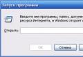
In addition, there is a possibility of using a dialog box Running program (Start - execute ...). So, to open the MS Excel program, it is enough to enter in the field Open Excel and press OK..

Microsoft Excel Working Window

The basic concepts of this

MS Excel application window consists of external (software) and internal (worker) windows. The inner window contains work sheet (there are several such sheets, they form book), representing a two-dimensional rectangular matrix. On the right and below are the scroll strips.

Each work sheet has a name that is displayed on label Sheet. With the help of labels, you can switch to other working sheets that are part of the book. To implement actions with a shortcut (renaming, color change, etc.) uses its context menu.

The work sheet consists of row and column. The columns are entitled with capital latin letters and, further, two-letter combinations. The entire work sheet may contain up to 256 columns numbered from A to IV. Rows are numbered sequentially numbered, from 1 to 65536 (the maximum permissible line number).

Cells and their addressing. At the intersection of columns and strings, table cells are formed. They are minimal elements for storing data. The designation of a separate cell combines the number of columns and strings (C7, DE234)

In the Excel window (see Figure), as in other MS Office software packages, the menu area is located below the header area, below the main panel (ruler) of the tool. Cell designation (its number) performs the functions of its address. The address of the cells are used when writing formulas that determine the relationship between the values \u200b\u200blocated in different cells.

One of the cells is always active and stands out for a frame of an active cell. Input and editing operations are always produced in the active cell. You can move the frame of the active cell using the cursor keys or the mouse pointer.

Range of cells. The data located in neighboring cells can be referenced in the formulas as a single whole. Such a group of cells is called the range. The most commonly used rectangular ranges formed at the intersection of a group of sequential rows and columns. The range of cells is indicated by pointing through the colon numbers of cells located in opposite corners of the rectangle (A1: B12).

If you want to highlight the rectangular range of cells, it can be drawn by pulling the pointer from one corner cell to the opposite diagonal. The frame of the current cell is expanding, covering the entire selected range. To select a column or a string of the whole, click on the column header (strings). Stretching the headlines pointer, you can select a few consecutive columns or rows.

Entering, editing and data formatting

A separate cell may contain data of different types (text, number, date, etc.) or remain empty. Having selecting the cell or range of cells, you can configure the format of the cells using the appropriate menu item or the context menu command. In addition, the data type placed in the cell is automatically determined when entering.

Enter text and numbers. Data entry is carried out directly into the current cell or string of the formula, located at the top of the program window under the toolbars. The entry place is marked with text cursor. If you start input by pressing alphanumeric keys, the data from the current cell is replaced by the text entered. If you click on the formula or twice on the current cell, the old cell content is not deleted and the ability to edit it appears. Included data in any case are displayed both in the cell and in the formula row.

To complete the input, saving the entered data, use the Enter button in the formula row or the Enter key. To cancel the changes made and restore the former cell value, use the Cancel button in the formula row or the ESC key. To clean the current cell or the dedicated range, the easiest to use the DEL key.

Formatting content of cells. Text data by default is aligned to the left edge of the cell, and the numbers are right. To change the data display format in the current cell or the selected range, use the format ® cell command. The tabs of this dialog box allow you to choose the data recording format, set the text direction and the alignment method, to determine the font and inscribe characters, control the display and view of the frame, set the background color.

Data sorting

The spreadsheets allow you to sort the data, i.e. produce their ordering. Data in this can be sorted ascending or descending. When sorting ascending, the data is built in the following order:

· Numbers are sorted by the smallest negative to the greatest positive number;

· The text is sorted in the following order: numbers, signs, Latin and Russian alphabets;

· Empty cells are always placed at the end of the list.

To sort the rows of the table, select the column whose data will be ordered. After sorting, the order of rows is changed, but their integrity remains.

You can carry out nested sorts, i.e. Sort the data sequentially in several columns. When sorting a string with the same values \u200b\u200bin the cells of the first column will be ordered by values \u200b\u200bin the cells of the second column, and the strings having the same values \u200b\u200bin the second column will be ordered by the values \u200b\u200bof the third column.

Search for data

In this, you can search for data in accordance with the specified conditions. Such conditions are called filter. As a result of the search, lines satisfy the specified filter will be found. Conditions are specified using relationship operations. For numerical data is operations equally (sign \u003d), less (sign<), more (sign\u003e), less or equal (combination of signs<=) и more or equal (combination of signs\u003e \u003d).

For text data, comparison operations are possible. equally, begin with (Compare the first characters), ends on (compared the last characters), contains (Symbols are compared in any part of the text).

You can search for data by entering the search terms for several columns. In this case, the filter will contain several conditions that must be performed simultaneously.

^

43.Invad, editing and data formatting

A separate cell may contain data related to one of three types: text, numberor formula,- And also remain empty. Program Excel when the working book is saved, only the rectangular area of \u200b\u200bworking sheets is recorded, adjacent to the upper left corner (cell A1) and containing all filled cells.

The type of data placed in the cell is determined automatically when entering. If this data can be interpreted as a number, program Excel Soand does. Otherwise, the data is considered as text. Entering the formula always starts with the symbol<=> (equality sign).

^ Enter text and numbers. Data entry is carried out directly to the current cell or in string formulaslocated at the top of the program window under the toolbars (see Fig. 12.2). The entry place is marked with text cursor. If you start input by pressing alphanumeric keys, the data from the current cell is replaced by the text entered. If you click on the formula or twice on the current cell, the old cell content is not deleted and the ability to edit it appears. Included data in any case are displayed both in the cell and in the formula row.

To complete the input, saving the entered data, use the Enter button in the formula row or the Enter key. To cancel the changes made and restore the former cell value, use the Cancel button in the formula row or the ESC key. To clean the current cell or selected range, the easiest to use the Delete key.

^ Formatting content of cells. Text data by default is aligned to the left edge of the cell, and the numbers are right. To change the data display format in the current cell or selected range, use the cell format command. The tabs of this dialog box allow you to choose a data recording format (the number of semicolons, indicating the monetary unit, the method of recording the date and so on), set the text of the text n method of alignment, to determine the font and character stacking, control the display and view of the frame, set the background color.

44. Tabular processors. Relative and absolute addiction (absolute link, relative reference, relative orientation rule. Create examples).

^ Absolute and relative links

By default, links to cells in formulas are considered as relative.This means that when copying the address formula, the links are automatically changed in accordance with the relative location of the original cell and the copy created.

Let, for example, in the B2 cell there is a link to the cell A3. In a relative view, it can be said that the link indicates a cell, which is located on one column to the left and one line below this. If the formula is copied to another cell, such a relative indication of the link will continue. For example, when copying the formula to the EA27 cell, the link will continue to indicate the cell located in the left and below, in this case, the DZ28 cell.

For absolute addressingaddresses of references during copying do not change, so that the cell on which the reference indicates is considered not tabular. To change the addressing method, when editing the formula, it is necessary to highlight the link to the cell and press the F4 key. The cell number elements using absolute addressing are preceded by $. For example, with sequential press keys F4, the cell number A1 will be written as a1, $ A $ 1, and $ 1 and $ A1. In the last two cases, one of the components of the cell number is considered as absolute, and the other - as relative.
^

45. Tabular processors. Copying formulas. Moving formulas. Create examples.

Formulas.Calculations in the Excel tables are carried out using formulas. The formula may contain numeric constants, cell references and Excel functions connected by mathematical operations. Brackets allow you to change the standard procedure for performing actions. If the cell contains a formula, then the current result of the calculation of this formula is displayed in the work sheet. If you make a cell current, then the formula itself is displayed in the formula row. The method of using the Formula in Excel program is that if the cell value does depends on other table cells, you should always use the formula, even if the operation can be easily performed in the "mind". This ensures that the subsequent editing of the table will not violate its integrity and the correctness of the calculations produced in it. Links to cells.The formula may contain links, that is, cell addresses, the contents of which are used in calculations. This means that the result of the calculation of the formula depends on the number located in another cell. The cell containing the formula is thus dependent. The value displayed in the formula is recalculated when the cell value changes to which the link indicates. A link to the cell can be set in different ways. First, the cell's address can be administered manually. Another way is to click on the desired cell or the selection of the band whose address is required. The cell or range is highlighted by a dotted frame. All Excel program dialog boxes that require specifying numbers or cell ranges, contain buttons connected to the corresponding fields. When you click on this button, the dialog box is folded to the lowest size, which facilitates the selection of the desired cell (range) by clicking or pulling. To edit formulas, double-click on the appropriate cell. At the same time, the cells (ranges), on which the value of the formula depends on the work sheet with color frames, and the links themselves are displayed in the cell and in the formula string in the same color. This facilitates editing and verifying the correctness of the formulas. Copying the contents of cells.Copying and moving the cells in the Excel program can be done by dragging or through the clipboard. When working with a small number of cells, it is convenient to use the first method when working with large ranges - the second. Dragging method. To make the drag and drop or move the current cell (dedicated range) along with the contents, the mouse pointer to the current cell (it takes the appearance of an arrow with additional arrows). Now the cell can be dragged into any place of the working sheet (the insertion point is marked with a pop-up tip). To select a method for performing this operation, as well as for more reliable control over it, it is recommended to use special drag and drop using the right mouse button. In this case, when the mouse button is released, a special menu appears in which you can choose a specific operation being performed. Apply the clipboard. Transferring information through the clipboard has certain features related to the complexity of control over this operation in the Excel program. First, it is necessary to highlight the copied (cut) range and give the command to its room in the clipboard: edit to copy or edit cut. Inserting data to the work sheet is possible only immediately after their room in the clipboard. Attempting to perform any other operation leads to the cancellation of the starting copy or movement process. However, data loss does not occur, since the "cut" data is removed from the location of their initial placement only at the time of the insertion. The insertion location is determined by specifying the cell corresponding to the upper left corner of the range placed in the clipboard, or by isolating the range, which in size exactly is equal to the copied (movable). Insert runs the Edit command to insert. To control the insertion method, you can use the edit command Special insert. In this case, the data insertion rules from the clipboard are set in the dialog that opens. Automation of input.Since tables often contain repeating or single-type data, the Excel program contains input automation means. The funds provided include: Autocomitics, autofill numbers and autofill formulas. Content. To automate text data entry uses the automatization method. It is used when entering a single column of the working sheet of text strings in the cell, among which there are repeated. During the input of text data in the next cell, the Excel program checks the compliance of the entered characters to the rows exhibiting in this column above. If an unambiguous coincidence is detected, the entered text is automatically complemented. Pressing the ENTER key confirms the operating operation, otherwise the input can be continued, not paying attention to the proposed option. You can interrupt the work of the automaticization tools, leaving a blank cell in the column. Conversely, to use the capabilities of the automaticization tools, the filled cells should go in a row, without intervals between them. Automatic autofills. When working with numbers, an autofill method is used. In the lower right corner of the current cell framework there is a black square - filling marker. When you hover on it, the mouse pointer (it usually has the appearance of a thick white cross) acquires the shape of a thin black cross. Dragging the filling marker is considered as the operation of the "reproduction" of the cell content in the horizontal or vertical direction. If the cell contains a number (including a date, a sum of money), then when dragging the marker, cells are copied or the filling of arithmetic progress occurs. To select a method of autofill, perform special drag and drop using the right mouse button. Let, for example, a cell A1 contains a number 1. Move the mouse pointer to the fill marker, press the right mouse button and drag the fill marker so that the frame covers the A1, B1 and C1 cells, and release the mouse button. If you now select Copy cells in the menu that opens, all cells contain a number 1. If you select the item to fill, then in the cells will be numbers 1, 2 and 3. To accurately formulate the conditions for filling the cells, you should give a command to fill the progression. In the Progression dialog that opens, the progression type is selected, the step value and the limit value. After clicking on the OK button, the Excel program automatically fills the cells in accordance with the specified rules. Autocomplete formulas. This operation is performed in the same way as autofill numbers. Its feature is to copy links to other cells. During the autofilement, the nature of references in the formula is taken into account: relative references are changed in accordance with the relative position of the copy and the original, the absolutes remain unchanged. For example, suppose that the values \u200b\u200bin the third column of the working sheet (column C) are calculated as the sums of values \u200b\u200bin the respective cells of the columns A and V. We introduce into the C1 cell formula \u003d A1 + B1. Now copy this formula by the method of autofill in all cells of the third table column. Due to the relative addressing, the formula will be correct for all cells of this column.

A separate cell may contain data related to one of three types: text, numberor formula -and also to remain empty. The Excel program, when saving a working book, records only a rectangular area of \u200b\u200bworking sheets, adjacent to the upper left corner (cell A1) and containing all filled cells.

The type of data placed in the cell is determined automatically when entering. If this data can be interpreted as a number, the Excel program does. Otherwise, the data is considered as text. The formula entry always begins with the "\u003d" symbol (equality sign).

Enter text and numbers. Data entry is carried out directly to the current cell or in string formulaslocated at the top of the program window directly under the toolbars (see Fig. 12.2). The entry place is marked with text cursor. If you start input by pressing alphanumeric keys, the data from the current cell is replaced by the text entered. If you click on the formula or twice on the current cell, the old cell content is not deleted and the ability to edit it appears. Included data in any case are displayed both in the cell and in the formula row.

To complete the input, saving the entered data, use the ENTER button in the formula row or the ENTER key. To cancel the changes made and restore the former cell value, use the Cancel button in the formula row or the ESC key. To clean the current cell or selected range, the easiest to use the Delete key.

Formatting content of cells. Text data by default is aligned to the left edge of the cell, and the numbers are right. To change the data display format in the current cell or the selected range, use the format command > Cells. The tabs of this dialog box allow you to choose the data recording format (number of semicolons, indicating the monetary unit, the method of recording the date, etc.), set the direction of the text and the method of alignment, to determine the font and characters, control the display and view of the framework, set the background color.

Calculations in spreadsheets

Formulas. Calculations in the Excel program tables are carried out using formulasThe formula may contain numerical constants, linkson cells I. functionsExcel connected by signs of mathematical operations. Brackets allow you to change the standard procedure for performing actions. If the cell contains a formula, then the current result of the calculation of this formula is displayed in the work sheet. If you make a cell current, then the formula itself is displayed in the formula row.

The rule of use of the formula in the Excel program is that if the cell value reallydepends on other table cells, is alwaysyou should use the formula, even if the operation can be easily performed in the "mind". It guarantees

Keywords:

• spreadsheets
• tabular processor
• column
• line
• cell
• range of cells
• book

Hundreds of years in the business sector, tables are used when performing cumbersome single type calculations. With their help, wages are calculated, various accounting systems are conducted, the cost of new goods and services is calculated, the amount of profit is predicted, etc. Such calculations have been performed by many experts to the end of the last century using calculators, manually enters the results obtained to the corresponding column columns . Such work required high time costs; On the correction of a minor error made by the calculation, the weeks left and even months.

The situation has changed dramatically with the advent of spreadsheets, which allowed the change in the source data to quickly solve a large number of typical calculated tasks.

Nowadays, spreadsheets are one of the software products most widely used in practice. With their help, users who do not have special knowledge in the field of programming, have the ability to determine the sequence of computing operations, perform various initial data transformations, represent the results obtained in graphical form.

5.1.1. Interface of spreadsheets

The most common tabl processors are Microsoft Excel and OpenOffice.org Calc. When you start any of them, a window is displayed, many elements of which you are well known to work with other programs (Fig. 5.1).

Fig. 5.1.
OpenOffice.org Calc table processor interface

String header Contains the name of the document, the program name and window control buttons.

Link menu Contains the names of group management teams of the spreadsheet combined by functional sign.

Toolbars contain pictograms to call the most frequently executed commands.

Workspace Tabular processor is a rectangular space separated by columns and lines. Each column and each line have designations (headers, names). The columns are designated from left to right Latin letters in alphabetical order; Single-bouquet, two-letter and three-letter names (A, B, C, etc., are used (A, B, s, and so on; after the 26th column, two-letter combinations of AA, AB, etc.) begins. Rows are numbered from top to bottom. The number of rows and columns in different tabular processors differently.

At the intersection of columns and rows, cells (cells) are formed in which data or operations performed above them can be recorded. The cell is the smallest structural unit of the spreadsheet. Each cell of the spreadsheet has a name made up from the literal name of the column and the line number, on the intersection of which it is located. The following names of the cells are possible: EL, K12, AB125 1. Thus, the cell name determines its address in the table.

1 In modern versions in Microsoft Excel, the cell position may be denoted by the letter R, followed by the line number, and the letter C, followed by a column number, for example R1C1.

The cell is the smallest structural unit of the spreadsheet, formed at the intersection of the column and string.

Table Cursor - Selected rectangle, which can be placed in any cell. The cell of the table that the cursor occupies currently is called the current cell. You can enter or edit data only in the current cell. In fig. 5.1 Current is C4 cell.

The address of the current cell and the data entered into it is reflected in the input row. In the input row, you can edit the information stored in the current cell.

Going in a row cells in a row, column or rectangle form range. When the range is specified, its initial and final cells are indicated, in the rectangular range - cells of the left upper and right lower corners. The largest range represents the entire table, the smallest is one cell. Examples of ranges: A1: A10, B2: C2, B2: D10.

The working area of \u200b\u200bthe table processor is otherwise called a sheet. The document created and stored in the table processor is called a book; It can consist of several sheets. Similar to sheets of accounting book, they can be pulled out, climbing on the labels located at the bottom of the window. Each page of the book user can specify a name based on the contents of this sheet.

The status bar displays messages about the current mode of operation of the table and the possible user actions.

5.1.2. Data in table cells

Content cells can be:

• text;
• number;
• formula.

Text is a sequence of any characters from a computer alphabet. Texts (inscriptions, headlines, explanations) are needed for the design of the table, the characteristics of the objects under consideration can be presented in the text form. You can change the contents of the cell with the text only by editing the cell. By default, the text is aligned in the cell along the left edge - by analogy with the letter of the letter from left to right.

Using numbers, the quantitative characteristics of the objects under consideration are set. This uses various numeric formats (Table 5.1). By default, a numeric format with two decimal places is used. To write numbers containing a large number of discharges that do not fit in the cell, an exponential (scientific) format is applied.

Table 5.1
Some numeric formats

Numeric data introduced into table cells are source data for calculations. Change numeric data by editing them. By default, the numbers are aligned in the cell along the right edge, which ensures the alignment of all the number of columns in the categories (the units are placed under units, dozens are under ten, etc.).

The whole and fractional parts of the real number are divided into electronic semicolons. When used in the recording of the number of points (as a separator of its integer and fractional parts), the number is interpreted as the date. For example, 9.05 is perceived as May 9, and 5.25 - as May 2025.

Formula - This expression (arithmetic, logical), specifying some sequence of data conversion actions. The formula always begins with the sign of equality (\u003d) and may include links (cell names), signs of operations (Table 5.2), functions and numbers.

Table 5.2.
Arithmetic operations
used in formulas

When writing formulas, there are rules similar to those adopted in programming languages. Examples of formulas:

To enter the cell name formula, it is enough to place a table cursor in the appropriate cell.

In the process of entering the formula, it is displayed both in the cell itself and in the input row. After the input is complete (pressing the ENTER key) in the cell displays the result of calculations according to this formula (Fig. 5.2). To view and edit a specific formula, it suffices to highlight the corresponding cell and to edit it in the input row.

Fig. 5.2.
Calculations according to the formula

When the source data changes in the cells, the names of which are included in the formula, the expression value is immediately recalculated, the result obtained is displayed in a cell with this formula.

5.1.3. Main modes of electronic tables

You can select the following electronic table modes:

• table formation modes;
• table display modes;
• computing modes.

Modes of formation of the spreadsheet. When working with tabular processors, documents can be viewed, which can be viewed, change, write to the external memory media for storage, print on the printer.

The formation of spreadsheet involves filling and editing the document. This uses commands that change the contents of the cells (clear, edit, copy), and commands that change the structure of the table (delete, insert, move).

The contents of the cells can be decorated using standard text design tools: changes in the font pattern, its size, drawing and alignment relative to the cell, the direction of writing. In addition, the user is available for the table of the table itself: association of cells, various ways of drawing boundaries between cells for printing.

Data, data format and cell registration parameters (font, fill color, border type, etc.) can be copied from some cells (cell ranges) to other cells (cell ranges) of the spreadsheet.

Table display modes. For the spreadsheet, the display mode of formulas or the display mode of values \u200b\u200bcan be set. The default mode of displaying values \u200b\u200bis enabled, and the values \u200b\u200bcalculated based on the contents of the cells are displayed on the screen. You can specifically set the display mode of the formula, in which the formulas themselves will be displayed instead of the results of the calculations (Fig. 5.3).

Fig. 5.3.
Fragment of the table in the formula display mode

To install the formula display mode in OpenOffice.org Calc.

1. run the service settings command-OpenOffice.org Calc view;
2. in the area, set the Formula Checkbox and click OK.

Other find out how the display mode is set in the table processor exhibiting at your disposal.

Computation modes. All calculations begin with a cell located at the intersection of the first string and the first column of the spreadsheet. Calculations are carried out in a natural order; If in the next cell is a formula, including the address of a not yet calculated cell, then the calculations on this formula are deposited until the value in the cell on which the formula depends will not be determined.

Each time you enter a new value in the cell, the document is recalculated again - the automatic conversion is performed by the formulas in which new data includes. In most tabular processors, it is possible to install manual recalculation: the table is recalculated only when submitting a special command.

In OpenOffice.org Calc, the selection of the computation mode is carried out using the service contents command-to-calculate automatically.

Alone, find out how the calculation mode is set in the table processor exhibiting at your disposal.

The most important thing

The spreadsheets (tabular processor) are an application program designed to organize table computing on a computer.

The cell is the smallest structural unit of the spreadsheet, formed at the intersection of the column and string. The cell content may be text, number, formula.

Texts (inscriptions, headlines, explanations) are needed for table design. Numeric data introduced into table cells are source data for calculations. In cells with formulas displays the results of calculations.

The formation of spreadsheets assumes filling, editing and formatting a document.

When you enter a new value in the cell, the document is crossed automatically, but manual recalculation mode can be installed.

For the spreadsheet, the display mode of formulas or the display mode of values \u200b\u200bcan be set.

Questions and tasks