Conditional formatting rules in Excel. A collection of formulas for conditional formatting
This tutorial with examples and videos will be devoted to conditional formatting - one of the most interesting and useful tools in Excel.
What is Conditional Formatting
So let's get down to business. Conditional formatting is a way to keep things as simple as possible excel programs... This method of processing information saves a lot of time and makes all calculations easier. You can make the program automatically perform many tasks that you previously did manually, killing days for it.
In addition, for your convenience, you can customize the work of Excel so that it immediately highlights the desired or important information in documents. In addition, such formatting will help to more clearly display information, quickly and efficiently create reports without using complex graphical models such as charts or graphs.
Let's take a look at more specific use cases conditional formatting... In order to apply it in Excel 10, in the "Home" section on the top panel of the program, you need to find the "Conditional Formatting" button. She is not hiding anywhere, so finding her will not be difficult. In order to activate this formatting, we need to select the area on the worksheet with which we will work. Keep in mind that before clicking the "Conditional Formatting" button and proceeding with it, you need to select a column, row or several such elements for which you want to use formatting.
So, the work area is highlighted, the button is pressed - what next? You will see a conditional formatting menu with the following items:
- Selection rules for the first and last values.
- Color scales.
- Optional: create, delete, rule management.
What to do about it? Let's go in order. This item, in turn, contains such standard functions, as
- More;
- Less;
- Equally;
- The text contains;
- Date;
- Repeating icons.
Working with these formatting models is not difficult at all. By clicking on any of them, you will open a small window where you will need to enter the data you need and select a color for highlighting the table cells that suit you.

- Click "Between" and in the new window that opens in the appropriate cells, enter the parameters from and to.
- Then specify the color that you want to highlight the options that suit you (let's say we have it "Light red fill and dark red text"). That is, if you work with a price column for cell phones, then enter the numbers of the minimum and maximum cost that suits you (let it be 50 and 100 for us).
- After you have confirmed that it is BETWEEN these values \u200b\u200b\\ u200b \\ u200bwant to start the search, the cells in the table will be highlighted accordingly and we will see ALL cells with a price from $ 50 to $ 10 colored in light red and with dark red text.
All this is not difficult at all when, in practice, start working with the program.
All the formatting methods in the Cell Selection Rules menu work in much the same way, so we will not dwell here.
Selection rules for the first and last values
The next point is before us. How it works? If you need to select the first or last few cells according to the entered data, then you are exactly where you need it. There is nothing more to explain, so let's move on to an example.


- By clicking "First 10 Items" we will bring up a window where you can control this formatting.
- Here we will indicate the number of cells that we need to select: originally it was named 10, but we only need 5, so we fix it in the corresponding field.
- Then we choose the formatting color: let us have it "Red border".
- Then the 5 cells with the highest values \u200b\u200bwill be highlighted with a red frame.
Let's go further. Everything is very simple here. You just need to select the column or line we need and click on the corresponding button. Then we will see how all the cells are more or less filled with color, depending on the values \u200b\u200binside them. It's like a real histogram.

- Press "Histogram" and select any model you like from the menu (they differ only in design).
- As a result, our column with the number of phones will change so that the entire cell of the largest digit will be filled with color completely, and all the rest will be filled in percentage to the maximum value.
Color scales
They allow us to color our cells in ascending or descending order of values \u200b\u200bin them. You only need to choose in what color range this will happen (for example, the maximum value is green, the minimum value is red, and all intermediate values \u200b\u200bwill be colored in the corresponding transition shades). We won't even give an example here.
The icons are needed to indicate the difference between the values \u200b\u200bin our column or row. It's a bit difficult to explain in theory, so let's jump straight to the examples.

- select "Icon Sets" and in the "Directions" section click on "5 colored arrows". Thus, in each cell of the field in which we work, one of 5 types of arrows will appear.
- Let's explain how they work: the entire range of values \u200b\u200bin the cells we have selected is 100%, and each arrow in turn is responsible for the numbers that enter every 20% in order. Suppose we have values \u200b\u200bfrom 0 to 100 in the column for the number of phone purchases.Then the first arrow (green up) will stand next to each value from 80 to 100, and the last (red down) - next to each value from 0 to 20. Accordingly, all intermediate arrows.
The percentage or the entire range can be configured in the Manage Rules menu, here you can also play around with the settings for other rules.
Conditional formatting in Excel is a great tool for quick visual analysis of data. It is much more convenient and easier to evaluate information in this way. Moreover, all this happens in automatic mode... The user does not need to think and compare values \u200b\u200bthemselves. The editor will do everything himself. In no formula can you do what this tool can.
In order to take advantage of this opportunity, you need to go to the "Home" tab and click on the "Conditional Formatting" button.
The main sections of this menu are:
- cell selection rules;
- rules for selecting the first and last values;
- histograms;
- color scales;
- sets of icons;
Let's take a closer look at these points. To do this, we will create some kind of table in which it will be possible to compare numeric values.
There are also a lot of different formatting options in this section. Let's analyze each of them.
More
- First, select a line. In this case, it will be the victims in the first mine.
- Then go to the "Home" tab and click on the "Conditional Formatting" button. In the menu that appears, click on the item "Cell selection rules". Then we select the "More" option.
- After that, a window will appear in which you need to specify a value for comparing the selected elements. You can drive in anything or click on any cell. Click on the average. This indicator is quite suitable for comparison.
- Immediately after that, the reference to the cell will be inserted automatically (and it will itself be highlighted with a dotted line). Click on the "OK" button to insert.
- As a result, we will see that the cells in which the value is greater than 27 are highlighted in a different color.
If you don't like the fill color of the cells, you can always change it. To do this, you need to choose any other coloring option at the stage of specifying the number for comparison.
If you don't like any of the proposed options, you can click on the "Custom format ..." item.
Immediately after that, a window will appear in which you can specify the cell format you need.
- Highlight a line. Click on the "Conditional Formatting" icon located on the "Home" tab. Select Cell Highlighting Rules and then Less.
- You will again be prompted to specify a cell for comparison. To do this, left-click on the desired cell.
- As a result, the required address will be substituted. Click on the "OK" button to save the settings.
- As a result of this, we see that all cells with a value less than 24 are highlighted in a different color.
- Select some line without formatting rules. We go to the same section of the menu, but this time select the "Between" item.
- Then the Excel editor himself will suggest some intermediate values. You can leave everything unchanged.
- Or substitute something of your own, which is more convenient for you. For example, more than 14, but less than 17. To save, click on the "OK" button.
- As a result, everything that is between these numbers was highlighted in a different color.
- Select another cell that is free of formatting. Do the same path on the toolbar and select the "Equal" item.
- We will be asked to provide a reference to a cell for comparison or a ready-made numeric value. Let's enter, for example, the number 18. Since it occurs in the highlighted line. To save, click on the "OK" button.
- Due to this, the cell that corresponds to the specified value has become highlighted in a different color.
- To check, you can try to change something. For example, let's take an adjacent cell. Let's fix 19 to 18. After pressing the Enter key, you will see the following.
We see that the background of the cells changes completely automatically.
The text contains
The above steps are only valid for numeric values. To work with text information you need to choose another tool.
- First of all, select a line with several numbers. Then, using the menu we are familiar with, select the "Text contains ..." item.
- As a result, a window will appear in which you need to specify a piece of text. It can be a letter or a number. For example, let's enter the number "2". Click on the "OK" button to save the formatting.
- As a result, cells with numbers 20 and 23 were highlighted, since both of them contain the number 2.
Similar manipulations can be done with time values.
- First, let's add a line in which we will write several dates. It is desirable that they go in a row. This will make it easier to compare.
- After that, select this entire line. Then go to the "Conditional Formatting" menu and select the "Date" item.
- Immediately after that, a window will appear in which you can select several options:
- yesterday;
- today;
- tomorrow;
- for the last 7 days;
- last week;
- this week;
- next week;
- last month;
- this month;
- next month.
- Let's take the "Tomorrow" option as an example. Click on the "OK" button to save.
- As a result, the field containing tomorrow's date will be highlighted in a different color.
- The current date as of this writing is February 25, 2018.
To demonstrate this conditional formatting, it is desirable to use a table with no other comparison rules. Next, you will need to follow these steps.
- Select in the table the main values \u200b\u200bthat need to be analyzed somehow.
- Click on the "Conditional Formatting" icon and select "Duplicate Values" in the "Cell Selection Rules".
- Immediately after that, a window will appear in which you can select two values:
- repetitive;
- unique.
In each case, a preview will be available so that you can determine exactly what you need. To save, click on the "OK" button.
In addition to the usual highlighting of specific numbers, it is possible to mark a certain number of elements in percentage or quantitative ratio. For this you need to do the following.
- Highlight the contents of the table. Then you need to click on the "Conditional Formatting" button, which is located on the "Home" tab. After that, select the "Rules for selecting the first and last values" item. As a result, you will be offered several selection options.
Let's consider each of them.
By selecting this item, you will see a window in which you will be asked to indicate the number of the first cells. Click on "OK" to save.
The countdown proceeds from the highest value to the lowest.
This means that if you need to select the first 10 cells in which the smallest numbers are located, then you need to select the "Last 10 elements" item.
As you enter the number of cells, you will see a preview. If you specify the number 1, then only 1 maximum value will remain.
Note that if there are two cells with the same highest number, both will be highlighted!
In this case, everything works practically on the same principle, only this time it is not a specific fixed number of cells that is highlighted, but only a certain percentage of them.
If you specify the number 10 (it is used by default), then you will see the following.
If you like this formatting rule, you need to click on the "OK" button. Otherwise, click on "Cancel".
Last 10 Items
As mentioned above, in this case, those cells are highlighted that contain the minimum data. The principle of entering is the same - you specify the required quantity and click on the "OK" button.
If you specify only 1 cell, but there will be several minimum numbers, then all will be selected (in our case, two).
The same principle, only this time a certain percentage of information is highlighted, and not an absolute amount.
This tool is very convenient when you need to sort information in relation to itself. That is, the Excel editor will calculate the average among the selected information itself and mark everything that is above this value. Everything happens automatically.
The principle of operation is similar in this case. Only this time, cells are marked in which information is stored less than the average value.
The data comparison methods described above used the solid fill method. Sometimes this is not very convenient.
For more advanced analysis of information, another tool is used - histograms. In this case, the fill can be of two types:
- gradient;
- solid.
Let's consider each of the proposed options.
Gradient fill
- The first step is to select the required rows and columns. Then click on the "Conditional Formatting" icon. After that, go to the "Histograms" section and select any of the offered fillings.
The default values \u200b\u200bare:
- green;
- red;
- orange;
- blue;
- purple.
When you hover over each of the options, you will see a preview.
This type of marking does not differ much from the one described above and is located in the same section.
The colors are the same.
If you didn't like any of the suggested items, you can specify your own formatting option.
Here you can configure:
- style;
- minimum and maximum value;
- appearance column.
A sample of what you've configured can be seen in the lower right corner.
If you want something more contrasting, you need to do the following.
- Highlight the table (basic information for data analysis). Click on the "Conditional Formatting" icon located on the "Main" tab on the toolbar. In the menu that appears, select the "Color Scales" item. As a result, a large list of 12 design options will appear.
- When you hover over each template, you will see a similar explanation.
When you hover over each of the icons, you will see a preview. This way you can choose the color scheme that you like the most.
If none of the suggested excel editor you didn't like it, you can always create something of your own. To do this, in the same section of the menu, click on the item "Other rules".
Immediately after that, you will see the following window. Here you can specify the start and end color. To save, just click on the "OK" button.
If you don't like color formatting, you can use the graphical method. To do this, you need to do the following.
- Select the main cells of the table.
- Click on "Conditional Formatting" in the toolbar.
- From the menu that appears, select the Icon Sets category.
- Right after that you will see a large list of different templates.
It should be noted that the editor automatically divides the data into several groups: minimum, average and maximum.
Possible options include (every time you hover over any icon, you will see a preview without saving the formatting rule):
- directions (an upward arrow will appear near large numbers; for medium numbers - to the right; downward direction corresponds to the minimum numbers);
- shapes (the color depends on the number in the cell - gray for the largest values);
- indicators (checkmark - high, exclamation mark - averages, and a cross - a minimum);
- estimates (the degree of filling an element depends on the number in the cell);
If you don't like any of the icons, you can create your own rule for filling cells.
In this case, you can independently specify the following parameters:
- icon style;
- your own version of the icon;
- boundary values \u200b\u200bfor icons;
Click on the "OK" button to save.
If your experiment failed and the manipulations you performed only spoiled the appearance of the table, then all this can be reversed in a fairly simple way.
- First, you need to select those elements whose conditional formatting needs to be disabled.
- Then click on the "Home" tab on the "Conditional Formatting" icon.
- After that select the "Delete rules" item.
- Next, click on "Remove rules from selected cells".
- If you want to delete everything, then select the second item - "Delete rules from the entire sheet."
- The result will be as follows. Everything will return to its former appearance.
The set of formatting methods can be changed at will. This is done as follows.
- Click on the "Conditional Formatting" button.
- Select "Manage Rules".
- There will be nothing in the appeared rules manager (if you didn’t select anything before calling this menu), because the "Current Fragment" item is selected by default.
- Select "This Sheet".
- As a result, you will see all the rules that are currently used in the document.
Deleting
In order to delete something, just select something from the list and click on the "Delete rule" button.
It is necessary to be very careful when performing such actions, since you will not be additionally asked if you are confident in your choice.
The change
Editing the rules is pretty straightforward. This is done as follows.
- Select any line.
- Click on the "Edit Rule" button.
- As a result, you will see the following window. By default, the "Format only cells that contain" type is selected.
- Here you can specify what exactly they contain:
- text;
- dates;
- empty;
- non-empty;
- errors;
- without mistakes.

In this tutorial, we'll go over the basics of applying conditional formatting in Excel.
With its help, we can highlight the values \u200b\u200bof tables in color according to specified criteria, search for duplicates, and also graphically “highlight” important information.
Excel Conditional Formatting Basics
Using conditional formatting, we can:
- paint values \u200b\u200bwith color
- change font
- format borders
It can be applied both to one and several cells, rows and columns. We can customize the format using conditions. Next, we will analyze in practice how to do this.
Where is the conditional formatting in Excel?
The "Conditional Formatting" button is located on the toolbar, on the "Home" tab:
How to do conditional formatting in Excel?
When applying conditional formatting, the system needs to set two settings:
- Which cells do you want to format;
- Under what conditions will the format be assigned.
Below, we'll look at how to apply conditional formatting. Let's imagine that we have a table with the dynamics of the dollar exchange rate in rubles for a year. Our task is to highlight in red those data in which the rate decreased in the previous month. So, let's follow these steps:
- In the data table, select the range for which we want to apply color highlighting:
- Let's go to the “Home” tab on the toolbar and click on the “Conditional Formatting” item. In the dropdown list, you will see several format types to choose from:
- Selection rules
- Selection rules for the first and last values
- Histograms
- Color scales
- Icon sets
- In our example, we want to highlight data with a negative value. To do this, select the type “Cell selection rules” \u003d\u003e “Less”:
Also, the following conditions are available:
- Values \u200b\u200bare greater than or equal to any value;
- Highlight text containing specific letters or words;
- Highlight duplicates;
- Highlight specific dates.
- In the pop-up window, in the “Format cells that are LESS” field, we will indicate the value “0”, since we need to highlight negative values \u200b\u200bwith color. In the drop-down list on the right, select the format that meets the conditions:
- To assign a format, you can use the pre-configured color palettes, and also create your own palette. To do this, click on the item:
- In the pop-up format window, specify:
- fill color
- font color
- font
- cell borders
- When finished, click “OK”.
Below is an example of a table using conditional formatting according to the parameters we specified. Data with negative values \u200b\u200bare highlighted in red:

How to create a rule
If the predefined conditions are not suitable, you can create your own rules. To configure, we will do the following steps:
- Let's select the data range. Click on the "Conditional Formatting" item in the toolbar. In the drop-down list, select the item "New rule":
- In the pop-up window, we need to select the type of rule to apply. In our example, the type "Format only cells that contain" is suitable for us. After that, let's set a condition to select data whose values \u200b\u200bare greater than “57” but less than “59”:
- Click on the "Format" button and set the format as we did in the example above. Click the "OK" button:

Conditional formatting by the value of another cell
In the examples above, we formatted the cells based on their own values. In Excel, it is possible to set the format based on values \u200b\u200bfrom other cells. For example, in the table with the dollar rate data, we can color the cells according to the rule. If the dollar rate is lower than in the previous month, then the value of the rate in the current month will be highlighted in color.
To create a condition for the value of another cell, follow these steps:
- Select the first cell for assigning the rule. Click on the "Conditional Formatting" item on the toolbar. Let's choose the “Less” condition.
- In the pop-up window, indicate the reference to the cell with which this cell will be compared. Choosing a format. Click the "OK" button.
- Re-select with the left mouse button the cell to which we assigned the format. Click on the "Conditional Formatting" item. Select “Manage rules” in the drop-down menu \u003d\u003e click on the “Edit rule” button:
- In the left field of the pop-up window, “clear” the link from the “$” sign. Click the "OK" button, and then the "Apply" button.
- Now we need to assign the customized format to the rest of the table cells. To do this, select the cell with the assigned format, then in the left upper corner on the toolbar, click on the "roller" and assign the format to the rest of the cells:
In the screenshot below, the data is highlighted in color, in which the currency rate has become lower compared to the previous period:

How to apply multiple conditional formatting rules to a single cell
It is possible to apply multiple rules to one cell.
For example, in the table with the weather forecast, we want to paint the temperature indicators with different colors. Highlighting conditions: if the temperature is above 10 degrees - green, if above 20 degrees - yellow, if above 30 degrees - red.
To apply multiple conditions to one cell, perform the following actions:
- Select the range with data to which we want to apply conditional formatting \u003d\u003e click on the item “Conditional formatting” on the toolbar \u003d\u003e select the selection condition “More ...” and indicate the first condition (if more than 10, then a green fill). We repeat the same steps for each of the conditions (more than 20 and more than 30). Despite the fact that we applied three rules, the data in the table is colored green:
Unformatted spreadsheets can be difficult to read. Rich text and cells can draw attention to certain parts of a spreadsheet, making them visually more visible and easier to understand.
There are many tools for formatting text and cells in Excel. In this lesson, you will learn how to change the color and style of text and cells, align text, and set custom formats for numbers and dates.
Text formatting
Many commands for formatting text can be found in the Font, Alignment, Number groups found on the ribbon. Group commands Font allow you to change the style, size and color of the text. You can also use them to add borders and fill cells with color. Group commands Alignment allow you to set the display of text in a cell both vertically and horizontally. Group commands Numberallow you to change the way numbers and dates are displayed.
To change the font:
- Select the desired cells.
- Click the Font command drop-down arrow on the Home tab. A dropdown menu will appear.
- Hover over different fonts. The selected cells will interactively change the font of the text.
- Select the font you want.
To change the font size:
- Select the desired cells.
- Click the drop-down arrow for the font size command on the Home tab. A dropdown menu will appear.
- Hover your mouse over different font sizes. The selected cells will interactively change the font size.
- Select the font size you want.

You can also use the Increase Size and Decrease Size commands to change the font size.

To use the bold, italic, underline commands:
- Select the desired cells.
- Click on the command bold (F), italic (K) or underlined (H) in the Font group on the Home tab.

To add borders:
- Select the desired cells.
- Click the command dropdown arrow boundaries on the home tab. A dropdown menu will appear.
- Select the desired border style.

You can draw borders and change line styles and colors using the border drawing tools at the bottom of the drop-down menu.
To change the font color:
- Select the desired cells.
- Click the drop-down arrow next to the Text Color command on the Home tab. The Text Color menu appears.
- Hover your mouse over different colors. On the sheet, the text color of the selected cells will interactively change.
- Choose the color you want.

The choice of colors is not limited to the dropdown menu. Select More Colors at the bottom of the list to access an expanded selection of Colors.
To add a fill color:
- Select the desired cells.
- Click the drop-down arrow next to the Fill color command on the Home tab. The Color menu appears.
- Hover your mouse over different colors. The fill color of the selected cells will interactively change on the sheet.
- Choose the color you want.

To change the horizontal alignment of text:
- Select the desired cells.
- Select one of the horizontal alignment options on the Home tab.
- Align text to the left: Aligns text to the left of the cell.
- Align Center:Aligns the text to the center of the cell.
- Align text to the right: Aligns text to the right of the cell.

To change the vertical alignment of text:
- Select the desired cells.
- Select one of the vertical alignment options on the Home tab.
- Top edge: Aligns text to the top of the cell.
- Align in the middle:Aligns text to the center of the cell between the top and bottom edges.
- Bottom edge: Aligns text to the bottom of the cell.

By default, numbers are aligned to the right and bottom of the cell, while words and letters are aligned to the left and bottom.
Formatting numbers and dates
One of the most useful functions Excel is the ability to format numbers and dates in different ways. For example, you might want to display numbers with a decimal separator, currency or percent symbol, etc.
To set the format for numbers and dates:

Numeric Formats

- General Is the default format for any cell. When you enter a number in a cell, Excel will suggest the most appropriate number format it thinks. For example, if you enter "1-5", the cell will display a number in the Short date format, "1/5/2010".
- Numerical formats numbers into decimal places. For example, if you enter "4" in cell, the cell will display the number "4.00".
- Monetaryformats numbers to display currency symbol... For example, if you enter "4" in cell, the cell will display the number as "".
- Financial formats numbers similar to Currency, but additionally aligns currency symbols and decimal places in columns. This format will make it easier to read long financial lists.
- Short date format formats numbers as M / D / YYYY. For example, the entry August 8, 2010 would be represented as "8/8/2010".
- Long date format formats numbers in the form Day of the week, Month DD, YYYY. For example, "Monday, August 01, 2010".
- Time formats numbers as HH / MM / SS and signature AM or PM. For example, "10:25:00 AM".
- Percentage formats numbers with decimal places and a percent sign. For example, if you enter "0.75" in a cell, it will display "75.00%".
- Fractional formats numbers as slash fractions. For example, if you enter "1/4" in a cell, then "1/4" will be displayed in the cell. If you enter “1/4” in a cell with the General format, “4-Jan” will be displayed in the cell.
- Exponential formats numbers to exponential notation. For example, if you enter "140000" in a cell, then the cell will display "1.40E + 05". Note: By default Excel will use the exponential format for a cell if it contains a very large integer. If you do not want this format, then use the Number format.
- Text formats numbers as text, that is, everything in the cell will be displayed exactly as you entered it. Excel uses this format by default for cells that contain both numbers and text.
- You can easily customize any format using the Other Number Formats item. For example, you can change the US dollar sign to a different currency symbol, specify the display of commas in numbers, change the number of decimal places displayed, etc.

Conditional formatting is one of the most useful EXCEL tools. Knowing how to use it can save the user a lot of time and effort.
Let's start exploring Conditional formattingfrom checking numeric values \u200b\u200bto more / less / equal / between versus numeric constants.
These rules are used quite often, therefore in EXCEL 2007 they are placed in a separate menu Cell selection rules.
These rules are also available through the menu Home / Styles / Conditional Formatting / Create Rule, Format only cells that contain.
Let's consider several tasks:
COMPARISON WITH A CONSTANT VALUE (CONSTANT)
Task1 A1: D1 with the number 4.
- enter into the range A1: D1 meaning 1, 3, 5, 7
- select this range;
- Conditional formatting on the value Less ();
- in the left field of the window that appears, enter 4 - we will immediately see the result of the application Conditional formatting.
- Click OK.

Task1.
COMPARISON WITH THE VALUE IN THE CELL (ABSOLUTE REFERENCE)
Let's complicate the previous task a little: instead of entering directly the value (4) as a criterion, we will enter a reference to the cell containing the value 4.
Task2... Compare values \u200b\u200bfrom the range A1: D1 with the number from the cell A2 .
- enter into the cell A2 number 4;
- select the range A1: D1 ;
- applicable to the selected range Conditional formatting on the value Less (Home / Styles / Conditional Formatting / Cell Highlighting Rules / Less);
- in the left margin of the window that appears, enter the cell reference A2 by clicking on the button located on the right side of the window (EXCEL by default uses the link $ A $ 2 ).
Click OK.
As a result, all values \u200b\u200bfrom the selected range A 1: D 1 will be compared to one cell $ A $ 2 ... Those values \u200b\u200bfrom A 1: D 1 which are smaller A 2 will be highlighted with the cell background fill.
The result can be seen in the example file on the sheet Task2.
To see how the formatting rule you just created is configured, click ; then double click on the rule or click the button Change rule... As a result, you will see the dialog box shown below.

PAIRED STRING / COLUMN COMPARISON (RELATIVE REFERENCES)
- enter in the cells of the range A 2: D 2 numerical values \u200b\u200b(you can consider them as criteria);
- select the range A 1: D 1 ;
- applicable to the selected range Conditional formatting on the value Less (Home / Styles / Conditional Formatting / Cell Highlighting Rules / Less)
- in the left margin of the window that appears, enter the relative reference to the cell A 2 (i.e. just A2 or mixed link A $ 2 ). Make sure there is no $ sign in front of column A.
Now each value in the line 1 will be compared with the corresponding value from the string 2 in the same column! The values \u200b\u200b1 and 5 will be highlighted because they are less than 2 and 6, respectively, located in row 2.
The result can be seen in the example file on the sheet Task3.

Attention!In the case of using relative links in the rules Conditional formatting it is necessary to keep track of which cell is active at the moment of calling the tool Conditional formatting .
Side note: On the importance of freezing the active cell when creating Conditional Formatting rules with relative links
When creating relative links in rules Conditional formatting, they "snap" to a cell that is active at the moment of calling the tool Conditional formatting.
TIP: To find out the address of the active cell (it is always one on the sheet), you can look in the field Name (located to the left of). In task 3, after selecting the range A1: D1 (the mouse button must be released), in, the address of the active cell will be displayed there A1 or D 1 ... Why are 2 options possible and what is the difference for conditional formatting rules?
Let's take a close look at the second step of solving the previous problem3 - selecting a range A 1: D 1 ... The specified range can be selected in two ways: select a cell A1 , then, without releasing the mouse button, select the entire range, moving right to D1 ; or, select a cell D1 , then, without releasing the mouse button, select the entire range, moving left to A1 ... The difference between these two methods is fundamental: in the first case, after completing the selection of the range, the active cell will be A1 , and in the second D 1 !
Now let's see how this affects the relative link conditional formatting rule.
If we selected the range in the first way, then by entering into the rule Conditional formatting relative cell reference A2 , we thereby told EXCEL to compare the value of the active cell A1 with value in A2 ... Because rule applies to range A 1: D 1 then B 1 will be compared with IN 2 etc. The problem will be solved correctly.
If when creating a rule Conditional formatting cell was active D1 , then its value will be compared with the cell value A2 ... And the value from A 1 will now compare with the value from the cell XFB2 (not finding cells to the left A 2 , EXCEL will select the most recent cell XFD for C1 , then the penultimate for B 1 and finally XFB2 for A1 ). You can verify this by looking at the created rule:
- select a cell A1 ;
- click Home / Styles / Conditional Formatting / Rules Management;
- now you can see that in relation to the range $ A $ 1: $ D $ 1 rule applies Cell value <XFB2 (or<XFB $ 2 ).

EXCEL displays a formatting rule ( Cell value

SELECTION OF LINE
SELECTION OF CELLS WITH NUMBERS
PRIORITY OF RULES
To check the rules applied to a range, use Conditional Formatting Rules Manager(Home / Styles / Conditional Formatting / Rules Management).

When two or more rules are applied to one cell Conditional formatting, the processing priority is determined by the order in which they are listed in Conditional Formatting Rules Manager... The rule higher in the list has a higher priority than the rule lower in the list. New rules are always added to the top of the list and therefore have a higher priority, but the order of the rules can be changed in the dialog using the arrow buttons Up and Down.
For example, there is a number 9 in a cell and two rules are applied to it Cell value\u003e 6 (format specified: red background) and Cell value\u003e 7(format set: green background), see the picture above. Because the rule Cell value\u003e 6 (format specified: red background) is higher, then it has a higher priority, and therefore the cell with a value of 9 will have a red background. On Check box Stop if true can be ignored, it is installed for backward compatibility with previous versions EXCEL that does not support the simultaneous application of multiple conditional formatting rules. Although it can be used to override one or more rules when using multiple rules set for a range at the same time (when there is no conflict between rules). You can learn more.
If a formatting rule applies to a range of cells, it takes precedence over manual formatting. Manual formatting can be done using the Format command from the Cells group on the Home tab. Manual formatting remains when you remove a conditional formatting rule.
CONDITIONAL FORMAT and CELL FORMAT
Conditional formatting does not change the Format applied to the cell (tab Main group Font, or press CTRL + SHIFT + F). For example, if the cell has a red fill in the cell and the Conditional Formatting rule is triggered, according to which the filling of this cell must be yellow, then the fill of the Conditional Formatting "wins" - the cell will be highlighted in yellow. Although the Conditional Format fill is applied over the Cell Format fill, it does not change (undo) it, and it is simply not visible.
DEBUGGING CONDITIONAL FORMATTING RULES
To test if the Conditional Formatting rule is being executed correctly, copy the formula from the rule to any blank cell (for example, the cell to the right of the Conditional Formatting cell). If the formula returns TRUE, then the rule is triggered, if FALSE, then the condition is not met and the cell formatting should not be changed.
Let's go back to problem 3 (see the section on relative links above). On line 4 we write the formula from the conditional formatting rule \u003d A1 Columns where the formula is TRUE will have conditional formatting applied, but FALSE will not. Before MS Excel 2010 for rules Conditional formatting you could not directly use links to other sheets or books. It was possible to get around this limitation by using. If in Conditional formattingyou need to make, for example, a cell reference A2
another sheet, you must first determine name for that cell and then refer to this name in the rule Conditional formatting... How it is implemented See example file on sheet Link from another sheet. All cells for which Conditional Formatting rules are set will be selected. On the menu Home / Styles / Conditional Formatting / Cell Selection Rules EXCEL developers have created a variety of formatting rules. In order not to reinvent the wheel, let's take a closer look at some of them. Now let's look at the newly created rule via the menu Home / Styles / Conditional Formatting / Managing Rules ... As you can see from the picture above, Conditional formatting you can set up to select not only cells, containing certain text, but also not containing, starting with and ending in specific text. Also, in case of conditions contains and does not contain application is possible. Let the cell again contain the word Drill... Select a cell and apply the rule The text contains... If we write down as a criterion r?, that word Drill will be highlighted. Criterion means: highlight words that contain syllables re, ra, re, etc. You need to understand that words with phrases will also be highlighted p2, pm, pQsince sign? means any character. If we write down as a criterion ??????
(select words with at least 6 letters), then, respectively, the word Drill will not be highlighted. You can, of course, achieve a similar result with the help of formulas with the functions MID (), LEFT (), DLSTR (), but this approach, you see, is faster. I also advise you to pay attention to the following rules from the menu Home / Styles / Conditional formatting / Rules for selecting the first and last values. Task4... Let there be 21 values, for convenience. Apply the rule Last 10 Items and set to highlight 3 values \u200b\u200b(items). See example file, sheet Task4. The words "Last 3 Values" mean the 3 lowest values. If there are repeats in the list, all matching repeats will be selected. For example, in our case, the third lowest value is 10 from the top. there are 10 more repeats in the list (there are 6 in total), then they will be highlighted as well Accordingly, the rules applied to our list: "Last 1 value", "Last 2 values", ... "Last 6 values" will lead to the same result - the selection of 6 values \u200b\u200bequal to 10. Applying the "Last 7 values" rule will result in the selection of all additional values \u200b\u200bequal to 11, since. The 7th lowest value is the first from top value 11. Similarly, you can create a rule to highlight the number of highest values \u200b\u200byou need by applying the rule First 10 elements. Consider another related rule Last 10%. Please note that in the picture above the "% of the selected range" checkbox is not checked. This checkbox is set either manually or when applying the rule Last 10%. This rule sets the percentage of the smallest values \u200b\u200bout of the total number of values \u200b\u200bin the list. For example, setting 20% \u200b\u200bof the latter will highlight the 20% of the lowest values. Let's try to set 20% of the last in our list of 21 values: six values \u200b\u200bwill be selected 10 (See example file, sheet Task4)... 10 is the minimum value in the list, so all its duplicates will be selected anyway. By setting the percentage from 1 to 33%, the selection will not change. Why? Setting, for example, 33%, we get that 6.93 values \u200b\u200bneed to be selected. Because you can select only an integer number of values, Conditional formatting rounds to the nearest integer, discarding the fractional part. But at 34%, it is already necessary to select 7.14 values, i.e. 7, and taking into account the repetitions of the value 11 following the 10th, 6 + 3 \u003d 9 values \u200b\u200bwill be selected. The creation of formatting rules based on formulas is limited only by the user's imagination. Here we will consider only one example, the rest are examples of use Conditional formatting can be found in these articles:; ; ; ... Let's suppose you need to select cells containing erroneous values: The same result can be achieved in a different way: Tatiana (not verified) Tatiana (not verified) Creator Me again. (not verified) Creator Tatiana (not verified) Creator Alexander 555 (not verified) Creator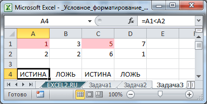
USE IN THE RULES OF LINKS TO OTHER SHEETS
SEARCH FOR CELLS WITH CONDITIONAL FORMATTING
OTHER PREDEFINED RULES


RULES USING FORMULAS

Comments