Microsoft Excel spreadsheet processor. Presentation on the topic "MS Excel" Presentation on the text editor Excel
Slide 1
Topic 8. Microsoft Excel spreadsheet Informatics For all specialties Institute IIIBS, IIKG department Kolmykova Oksana VladimirovnaSlide 2
 Spreadsheets Spreadsheets are a class of programs that allow you to present tables in electronic form and process their data. The use of spreadsheets simplifies the work with data and allows you to get results without manual calculations or special programming. The main advantage of a spreadsheet is the ability to instantly automatically recalculate all data linked by formula dependencies when the value of any component of the table changes.
Slide 3
 EXCEL functionality The Excel spreadsheet processor allows you to: Solve mathematical problems: perform tabular calculations (including as a regular calculator), calculate values \u200b\u200band explore functions, plot functions (for example, sin, cos, tg, etc.), solve equations, work with matrices and complex numbers, etc. 2. To carry out mathematical modeling and numerical experimentation What happens if? How to do that? 3. Conduct statistical analysis, forecasting (decision support) and optimization. 4. Implement the functions of the database input, search, sorting, filtering (selection) data analysis.
Slide 4
 Functionality of EXCEL 5. Enter passwords or protect some (or all) table cells, hide (hide) table fragments or the entire table. 6. Present data in the form of charts and graphs. 7. Enter and edit texts, as in a word processor, create pictures using the graphics editor Microsoft Office. 8. Carry out import-export, data exchange with other programs, for example, insert text, pictures, tables prepared in other applications, etc. 9. Carry out multi-table connections (for example, combine reports of branches of companies).
Slide 5
 Basic Spreadsheet Concepts A MS Excel document is called a workbook. A workbook is a collection of worksheets. Each worksheet has a title that appears on the sheet tab. The worksheet table space is composed of rows and columns. the maximum number of columns is 256 rows are numbered from 1 to 65536.
Slide 6
 Entering data into cells You can enter data of various types into cells, including: Text - any data on which there is no need to perform arithmetic operations; Numbers - numeric values \u200b\u200bin various formats: 36 45.23 2E-2 Date / Time 18.04.01; 18-Apr-01; Formulas (including functions) \u003d 12 + 34 \u003d A2 + B2
Slide 7

Slide 8

Slide 9

Slide 10

Slide 11

Slide 12

Slide 13
 Building charts Selecting data. If the data forms a single rectangular range, then it is convenient to select them using the Data Range tab. If the data does not form a single group, then the information for drawing individual data series is set on the Series tab.
Slide 14
 Building diagrams Chart design. On the design tabs, you can set: the title of the diagram, the axis labels (the Titles tab); display and labeling of axes (Axes tab); displaying a grid of lines parallel to the coordinate axes (the Gridlines tab); description of the plotted charts (Legend tab); displaying labels corresponding to individual data elements on the chart (Data Labels tab); presentation of the data used in the construction of the graph in the form of a table (tab Data table).
Slide 15
 Building diagrams Placing a diagram. Specifies whether to use a separate sheet or one of the available ones for placement.
Slide 16

Slide 17
 Using Standard Functions A function in EXCEL is defined as predefined formulas that perform calculations on specified values, called arguments, and in a specified order. Standard functions are used in spreadsheets only in formulas. A function call consists in specifying the function name in the formula, after which the list of parameters is indicated in brackets: \u003d SUM (D2: D7) Separate parameters in the list with a semicolon. \u003d SUM (D2: D7; B2: B7; C2: C7) The parameter can be a number, cell address, or an arbitrary expression, which can also be calculated using functions.
Slide 18
 Using the Function Wizard The Function Wizard makes it easy to enter and select the desired function. In the Category list, a category is selected to which the function belongs in the Function list - a specific function of this category. The function wizard is called using a special icon on the toolbar.
Slide 19
 Data processing operations in spreadsheets. Sort Sort is the sorting of data in ascending or descending order. To perform sorting, you need to do the following: Select any non-empty cell in the table. Run the command Data - Sort. The Sort Range dialog box appears. In the Sort list, specify the field by which the table will be sorted. If the check box Identify fields by labels (first row of the range) is selected, then the drop-down list will contain the names of the columns contained in row1. If the option Identify fields by designations of sheet columns is checked, then the first line is considered as an ordinary record, and not as a series of field names. In this case, in the drop-down list, the names of the columns will be shown as follows: Column A, Column B, Column C, etc. Select sorting order: ascending or descending. To sort by several fields at once, use the Then By and Last By, lists. You need to specify in them the fields by which you will need to sort the data if the values \u200b\u200bof the previous fields match. Click the OK button to sort the data in that order. You can quickly sort data using the buttons on the Sort Ascending toolbar to sort values \u200b\u200bin ascending order, or Sort Descending to sort values \u200b\u200bin descending order.
Slide 20

Slide 21
 Data filtering List filtering - displaying only those records (rows) that meet a certain criterion (condition)
Slide 22

Slide 23

Slide 24
 Definitions Spreadsheets are a class of programs that allow you to present tables in electronic form and process their data. Spreadsheet is the most common and powerful technology for professional data manipulation.
Slide 25
 Basic operations Solve mathematical problems: perform calculations and investigate functions, build graphs of functions, solve equations, work with matrices and complex numbers, etc. Perform mathematical modeling and numerical experimentation. Perform statistical analysis, forecasting and optimization. Implement database functions - input, search, sorting, filtering (selection) and data analysis.
Slide 26
 Basic Operations Enter passwords or protect table cells, hide parts of a table or the entire table. Present data in the form of charts and graphs. Carry out import-export, exchange data with other programs. Carry out multi-tabular communications. Prepare speeches, reports and presentations thanks to the built-in presentation mode.
Slide 27
 ... Basic Concepts An MS Excel document is called a workbook. A workbook is a set of worksheets, each of which has a tabular structure and can contain one or more tables. Each worksheet has a title that appears on the sheet tab displayed at the bottom of the worksheet.
Slide 28

Slide 29
 Basic Concepts The table space of a worksheet is composed of rows and columns. The columns are headed with Latin letters (maximum number of columns is 256). Lines are sequentially numbered from 1 to 65536
Slide 30

Slide 31
 At the intersection of columns and rows, table cells are formed. Each cell has an address that combines the column and row numbers at the intersection of which it is located. Range of cells - data located in adjacent cells, which can be referenced as a whole
Slide 32

Slide 33
 Data types Text - any data on which there is no need to perform arithmetic operations; Numbers - numeric values \u200b\u200bin various formats: 36; 45.23; 2E-2; Date / Time - 04/18/01; 18-Apr-01; Formulas (including functions) - \u003d 12 + 34; \u003d A2 + B2. etc.
Slide 34
 Calculations in ET A formula is a mathematical expression that starts with an equal sign and can contain numeric constants, cell references, and Excel functions connected by mathematical operation signs (+, -, *, /, ^)
Slide 35
 Calculations in tables Calculations in tables are performed using formulas. The formula can contain numeric constants, cell references and Excel functions, connected by signs of mathematical operations + addition - subtraction * multiplication / division ^ exponentiation
Slide 36
 In the lower right corner of the cell where the formula was entered is the fill marker. When you hover over it, the mouse pointer becomes a thin black cross. Dragging the handle lets you copy the formula horizontally or vertically. This method is called autocomplete.
Slide 37
 Formatting cells To format spreadsheets, you need to: select the appropriate cell or select a range of cells; select the menu item Format ~ Cells ~; select the appropriate tab: Sheets with tabs are used to perform the following functions: Number - setting the formats of numbers; Alignment - formatting the position of data in cells; Font - formatting data fonts; Border - selection of table frame; View - selection of the filling method for cells; Protection - protects cells and hides formulas.
Slide 38
 Charting in Spreadsheets Choosing a chart type depends on both the nature of the data and how you want to present it. The most commonly used chart types are: Pie. Used to display the relative relationship between parts of a whole. Bar graph. Used to illustrate the relationship of individual data values. Ruled. Used to compare values \u200b\u200bat a specific point in time. Schedule. Used to display trends in data at regular intervals. With areas. Used to emphasize the amount of change over a period of time.
Slide 39
 Key terms used in charts A data series is a group of cells within one column or one row. Categories - reflect the number of items in a row. Figure 7 shows 6 categories for each series (data for January, February, March, etc.) Legend - identifies individual chart elements. Grid - continuation of the division of the axes, improves the perception and analysis of the data on the chart
Slide 40
 Building diagrams for building a diagram use the Diagram Wizard, launched by clicking the Diagram Wizard button on the standard toolbar. Building diagrams consists of several stages: Choosing a diagram type. At this stage, the shape of the diagram is chosen. Type on the Standard or Custom tab View Building diagrams Chart design. On the design tabs, you can set: title of the chart, axis labels (the Titles tab); display and labeling of axes (Axes tab); displaying a grid of lines parallel to coordinate axes (the Gridlines tab); description of the plotted graphs (Legend tab); displaying labels corresponding to individual data elements on the chart (Data Labels tab); presentation of the data used in the construction of the graph in the form of a table (tab Data table). Using Standard Functions A function in EXCEL is defined as predefined formulas that perform calculations on specified values, called arguments, and in a specified order. Standard functions are used in spreadsheets only in formulas. The function call consists in specifying the function name in the formula, after which the list of parameters is indicated in parentheses: \u003d SUM (D2: D7) Separate parameters in the list with a semicolon. \u003d SUM (D2: D7; B2: B7; C2: C7) The parameter can be a number, cell address, or an arbitrary expression, which can also be calculated using functions. Data processing operations in spreadsheets. Sort Sort is the sorting of data in ascending or descending order. To perform sorting, you need to do the following: Select any non-empty cell in the table. Run the command Data - Sort. The Sort Range dialog box appears. In the Sort list, specify the field by which the table will be sorted. If the check box Identify fields by labels (first row of the range) is selected, then the drop-down list will contain the names of the columns contained in row1. If the option Identify fields by designations of sheet columns is checked, then the first line is considered as an ordinary record, and not as a series of field names. In this case, in the drop-down list, the names of the columns will be shown as follows: Column A, Column B, Column C, etc. Select sorting order: ascending or descending. To sort by several fields at once, use the Then By and Last By, lists. You need to specify in them the fields by which you will need to sort the data if the values \u200b\u200bof the previous fields match. Click the OK button to sort the data in that order. You can quickly sort data by using the buttons on the Sort Ascending toolbar to sort values \u200b\u200bin ascending order or Sort Descending to sort values \u200b\u200bin descending order. * Use of presentation materials The use of this presentation can be carried out only subject to the requirements of the laws of the Russian Federation on copyright and intellectual property, as well as taking into account the requirements of this Statement. The presentation is the property of the authors. You may print a copy of any part of the presentation for your personal, non-commercial use, but you may not print any part of the presentation for any other purpose or, for any reason, make changes to any part of the presentation. The use of any part of the presentation in another work, whether in print, electronic or otherwise, as well as the use of any part of the presentation in another presentation by reference or otherwise is allowed only after obtaining the written consent of the authors.
Spreadsheet - this is the computer equivalent of a regular table, consisting of rows and columns, at the intersection of which are cells containing numerical information, formulas, text.

MICROSOFT EXCEL PROGRAM allows:
- form data in the form of tables;
- calculate the contents of cells by formulas, while using more than 150 built-in functions;
- present data from tables in graphical form;
- organize data in a structure similar in capabilities to a database.

STARTING THE PROGRAM
To start the program, you can use the main menu command
Windows Start - All Programs - Microsoft Office - Microsoft Excel
or a shortcut on the desktop
and quick access.

Screen view
NORMAL - the most convenient for most operations.
PAGE LAYOUT - handy for final table formatting before printing.
PAGE - shows only available pages
To switch between modes, use the corresponding menu items View or by pressing the corresponding buttons

the main thing - contains functions for formatting and editing table data and the table itself (font, cell format, adding rows ...)
Insert - contains functions for inserting various objects into the book (text, illustration, diagram ...)
Page layout - contains functions for setting page parameters

Formulas - adds formulas to the table and assigns names to cells.
Data - work on data (insert, sort, filter ...)
Peer review - contains functions for checking spelling, inserting notes and protecting the book
View - functions for setting the appearance of the book window

ORGANIZATION OF DATA IN THE PROGRAM
The program file is a so-called Working Book ,
or working folder.
Each workbook can contain
more than 256 Worksheets .
By default, the Excel version contains
3 worksheets.
The sheets can contain both interconnected,
and completely independent information.
The worksheet is
blank for the table.
Column - all cells located in the same vertical row of the table. Column headings are specified by letters of the Latin alphabet, first from A to Z, then from AA to AZ, from BA to BZ, etc.
Row - all cells located at the same horizontal level. Row headers are represented as integers, ranging from 1 to 65,536.
A cell is a primitive spreadsheet object located at the intersection of a column and a row. The cell address is determined by its location in the table, and is formed from the column and row headers at the intersection of which it is located. The column heading is written first, followed by the row number. For example: A3, D6, A9, etc. A cell is called active when information (text, number, formula) is entered into it.
A range of cells is a group of adjacent cells that can consist of one cell, row (or part of it), column (or part of it), as well as a collection of cells that enclose a rectangular area of \u200b\u200bthe table. The range of cells is specified by specifying the addresses of the first and last cells, separated by a colon. For example: the address of the range formed by part of line 3 - E3: G3; the address of a range that looks like a rectangle with the starting cell F5 and the ending cell G8 - F5: G8.


DATA INPUT
To enter data into a cell, make it active and enter:
number (it is automatically right-aligned);
text (it is automatically left aligned);
formula (in this case, the cell will contain the result of calculations, and the expression will be highlighted in the formula bar, starting with the \u003d sign).
After entering text or a number with the cursor keys, you can move to an adjacent cell; when entering a formula, pressing the key will get the result of the calculation.
To correct information in an already filled cell, make it current, then press the key or double-click on the cell.
Press the key to exit the correction mode.

DISPLACEMENT -
Between cells:
Cursor buttons
- cursor (mouse)
- enter key
Between sheets:
- click on the sheet tab
- horizontal scrolling buttons

SELECTION OF FRAGMENTS OF THE TABLE
To perform an action on a group of cells,
they must be selected first.
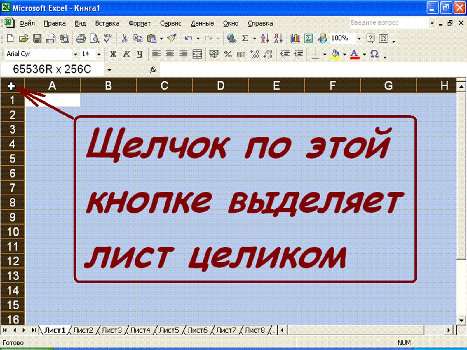
Wherein background all cells except the first will be painted over black color. But the cell that is not filled will also be selected.
To highlight ONE LINE , place the mouse pointer on the line number on the coordinate column .
To highlight multiple lines we move along the coordinate column, without releasing the left key .
To highlight ONE COLUMN , place the mouse pointer on a letter on the coordinate line.
To highlight multiple columns we move along the coordinate line, without releasing the left key .
To select several cells, move through the table with the left key pressed.
The selection is removed by clicking anywhere on the screen.

Working with data
Test input:
Select a cell and enter
or select a cell, position the cursor in the formula bar and enter
cancel input accept input call function wizard

Freezing regions
To anchor the upper horizontal area - indicate the line above which you want to anchor the area.
To freeze the left vertical region - select the column to the left of which you want to freeze the region.
To freeze both areas - select the cell located to the right and below the place where you want to split the sheet.

FONT CHANGE AND ALIGNMENT
Menu THE MAIN THING or tab FONT
Do not forget to select the required cells before making changes

SETTING Dividing lines

SET BACKGROUND COLOR AND FONT
Changes the active cell or selection

INSERTING CELLS, ROWS AND COLUMNS
MENU THE MAIN THING
Inserts or removes the selected number of cells, rows, or columns

Worksheet Management:
Actions
Sequence of execution
Rename sheet
Double click, enter a name, Enter
Add sheet
Delete sheet
Paste Sheet
Delete Sheet
Move sheet
Dragging with the mouse to the location indicated by the triangle
Copy sheet
Drag while pressed Ctrl
Change label color
Format Arrange sheet Label color
CONTEXT MENU functions

FORMATTING ROWS AND COLUMNS
menu
command
the main thing
Format - Cell - Cell Size (Width, Fit, Hide, Show)
the main thing
Alignment - Merge and Center (Width, Fit Width, Hide, Show)
CONTEXT MENU functions
TRANSPORTATION
Rotate the table 90 degrees
Home - Copy - Transport (Paste Special - Transport)

Change column width and row height
WIDTH: cursor in the title bar at the border of adjacent columns - double-headed arrow - drag
HEIGHT: mouse cursor on the border of adjacent lines - double-sided arrow - dragging
(the selected area also changes)

PAGE SETTINGS
MENU: Page Layout
Fields
Orientation
The size
Print area

SAVING YOUR WORKBOOK
In the window that appears, open the folder in which the file will be saved, in
enter the file name
(extension is defined by default as * .xls).

SORTING
Alphabetical arrangement of text and data:
THE MAIN IS EDITING
PAGE BREAKING
Setting the end of the page:
select the intended top-left cell of the new page
PAGE PARAMETERS - BREAKS

DATA FORMATS
MAIN - Cell - Format - Cell Format
Change bit depth:
Main - Number

Copying
Copy the contents of a cell to another cell.
Copies the contents of a cell to a range of cells. In this case, the contents of the original
cells are copied to each cell of the corresponding range.
Copy the contents of a range to another range. Moreover, both ranges
must have the same dimensions.
When you copy a cell, the contents of the cell, formatting attributes and notes (if any) are copied, the formulas are modified.

Removing content
Select a cell or range;
a) grab the fill handle, drag up or left and release the button
b) press;
c) Editing - Clear.

COPY METHODS
1 ... Using the clipboard
Highlight.
Toolbar button,
Context menu.
Place the table cursor in the upper left corner of the destination range and execute
insert operation (Button, Context Menu)
When pasting from the clipboard, all values \u200b\u200bin the cells of the destination range are erased without any warning
(apply cancellation if necessary)

COPY METHODS
2. Dragging D&D
Highlight.
Move the mouse pointer to the selection frame, when it turns into an arrow, click (a + sign will be added to the pointer), drag to a new location.
If the mouse pointer does not take the shape of an arrow when dragging, then Tools - Options - Edit tab - mark Dragging cells.

MOVEMENT
Moving a range is done in the same way as copying (without dragging and using the Cut command for clipboard).
It is very convenient to use special drag and drop (with the right mouse button pressed). This provides additional options that can be selected from the menu.


aUTOSUM button
Menu command
The formula you create
Summarize
Appointment
SUM (address_range)
Mean
AVERAGE (range_address)
Sum of all numbers in the range
Number
Maximum
Average
ACCOUNT (address_range)
MAX (address_range)
Amount of numbers
Minimum
Largest number in range
MIN (address_range)
The smallest number in the range


Task 1: Create a table using a sample, make a calculation using autosum and autocomplete.
Save as TRAVEL

Assignment 2:
- Create a document in MS Excel , name - Task 2
- Make a row of 10 numbers.
- Count:
- Amount The average Number Maximum Minimum
- Amount The average Number Maximum Minimum
- Amount The average Number Maximum Minimum
- Amount The average Number Maximum Minimum
- Amount
- The average
- Number
- Maximum
- Minimum
- Make a decision in the form:
- Save your changes to your document.
You should get such answers.


Slide 2
- History and development trends
- Basic concepts
- Launching MS Excel
- Introducing MS Excel Screen
- Standard pane and format pane
- Other elements of the Microsoft Excel window
- Working with sheets and books
Slide 3
Purpose and scope of table processors
- Practically in any area of \u200b\u200bhuman activity, especially when solving economic planning problems, accounting and banking, etc. it becomes necessary to present data in the form of tables.
- Spreadsheets are designed to store and process information presented in tabular form.
Slide 4
- Table processors provide:
- input, storage and correction of data;
- design and printing of spreadsheets;
- friendly interface, etc.
- Modern table processors provide a variety of additional features:
- the ability to work in a local network;
- the ability to work with three-dimensional organization of spreadsheets;
- development of macros, setting up the environment for the needs of the user, etc.
Slide 5
History and development trends
- The idea of \u200b\u200bcreating a table came from a student of Harvard University (USA) Dan Bricklin in 1979. Performing boring economic calculations using a ledger, he and his friend Bob Frankston, who knew about programming, developed the first spreadsheet program they called VisiCalc.
- A significant new step in the development of spreadsheets is the appearance in 1982. in the software market Lotus 1-2-3. Lotus raises its sales to $ 50 million in its first year. And it becomes the largest independent software company.
Slide 6
- The next step is the appearance in 1987. spreadsheet processor Excel from Microsoft. This program offered a simpler graphical interface in combination with pull-down menus, greatly expanding the functionality of the package and improving the quality of the output.
- The spreadsheet processors on the market today are capable of handling a wide variety of economic and other applications and can satisfy virtually any user.
Slide 7
Basic concepts
- A spreadsheet is the automated equivalent of a regular spreadsheet, where cells contain either data or the results of a formula calculation.
- The working area of \u200b\u200ba spreadsheet consists of rows and columns that have their own names. The names of the lines are their numbers. Column names are Latin letters.
- A cell is an area defined by the intersection of a column and a row in a spreadsheet and has its own unique address.
Slide 8
- The cell address is determined by the name (number) of the column and the name (number) of the row at the intersection of which the cell is located.
- Link - specifying the address of the cell.
- A block of cells is a group of contiguous cells identified by an address. A block of cells can consist of one cell, row, column, or a sequence of rows and columns.
- The address of a blocking cell is specified by specifying the links of its first and last cells, between which a separator character is placed - a colon or two periods in a row.
Slide 9
Introduction to MS Excel spreadsheet processor
- MS Excel spreadsheet is used for data processing.
- Processing includes:
- carrying out various calculations using the powerful apparatus of function and formulas;
- study of the influence of various factors on the data;
- solving optimization problems;
- obtaining a sample of data that meets certain criteria;
- construction of graphs and diagrams;
- statistical analysis of data.
Slide 10
Launching MS Excel
- When MS Excel starts, the “Book 1” workbook appears on the screen, containing 16 worksheets.
- Each sheet is a table.
- In these tables, you can store data with which you will work.
Slide 11
Ways to launch MS Excel
- 1) Start - Programs - Microsoft Office - MicrosoftExcel.
- 2) In the main menu, click on the "New Document" Microsoft Office, and on the Microsoft Office panel - the icon "New Document".
- The "Create document" dialog box appears on the screen. To start MS Excel, double-click the "New Book" icon
- 3) Double-click the left mouse button on the shortcut with the program.
Slide 12
MS Excel screen
- Standard panel
- Formatting bar
- Main menu bar
- Column headers
- Row headers
- Status bar
- Scroll bars
- Title bar
Slide 13
- Name field
- Formula bar
- Tab scroll buttons
- Sheet tab
- Label split marker
- Input buttons,
- cancellation and
- function wizards
Slide 14
Toolbars
- Toolbars can be arranged one after another on the same line. For example, when you first start a Microsoft Office application, the Standard toolbar is next to the Formatting toolbar.
- Placing multiple toolbars on the same line may not have enough room to display all buttons. In this case, the most frequently used buttons are displayed.
Slide 15
- Standard panel
- serves to perform such operations as: saving, opening, creating a new document, etc.
- Formatting bar
- serves to work with text, for example, aligning the center, right and left, to change the font and style of writing the text.
- Standard panel
- Format bar
Slide 16
Main menu bar
- It includes several menu items:
- file - for opening, saving, closing, printing documents, etc .;
- edit - serves to cancel input, re-enter, cut copying of documents or individual sentences;
- view - serves to display different panels, as well as page layout, task pane output, etc.;
- insert - serves to insert columns, rows, diagrams, etc .;
- format - serves for formatting text;
- service - serves to check spelling, protection, settings, etc .;
- data - serves for sorting, filtering, data validation, etc .;
- window - serves to work with a window; help to display help about a document or the program itself.
Slide 17
- Row and column headings are needed to find the cell you want.
- The status bar shows the states of the document.
- Scroll bars are used to scroll the document up and down, right and left.
- Column headers
- Row headers
- Status bar
- Scroll bars
Slide 18
- Name field
- Formula bar
- Tab scroll buttons
- Sheet tab
- Label split marker
- Input buttons,
- cancellation and
- function wizards
- The formula bar is used to enter and edit values \u200b\u200bor formulas in cells or charts.
- The name field is the window to the left of the formula bar that displays the name of a cell or range of cells.
- Tab Scroll buttons scroll the workbook tabs.
Slide 19
Working with sheets and books
- Creation of a new workbook (file menu - create or via the button on the standard toolbar).
- Saving a workbook (menu file - save).
- Opening an existing book (file menu - open).
- Protecting a book (sheet) with a password (the "protect" command from the service menu).
- Rename a sheet (double click on the sheet name).
- Sets the color of the sheet label.
- Sort sheets (menu data - sort).
- Insert new sheets (insert - sheet)
- Insert new lines (select a line and right-click - add).
- Changing the number of sheets in the book (menu "service", command "parameters", set the switch in the field "sheets in a new book").
Slide 20
Final slide
- Tabular Processor Basics
- Purpose and scope of table processors
- History and development trends
- Basic concepts
- Introduction to MS Excel spreadsheet processor
- Launching MS Excel
- Ways to launch MS Excel
- MS Excel screen
- Toolbars
- Main menu bar
- Working with sheets and books
View all slides


1 of 17
Presentation on the topic: Microsoft Excel
Slide No. 1

Slide Description:
Slide No. 2

Slide Description:
Everything about formulas A formula performs calculations of the corresponding tasks and displays the final result on a sheet; You can use numbers, arithmetic signs, and cell references in Excel formulas; The formula ALWAYS starts with an equal sign (\u003d); By default, formulas are not displayed on the screen, but you can change the operating mode of programs to see them; Formulas can include calls to one or more functions; Spaces are not allowed in formulas; The length of the formula must not exceed 1024 elements; You cannot enter numbers in date and time of day formats directly into formulas. They can only be entered in formulas as text enclosed in double quotes. Excel converts them to the corresponding numbers when calculating the formula.
Slide No. 3

Slide Description:
Entering a formula Click the cell where you want to enter a formula; Enter an equal sign - the required beginning of the formula. Enter the first argument, a number or a cell reference. The address can be entered manually or inserted automatically by clicking the desired cell; Enter an arithmetic sign; Enter the following argument; Repeating steps 4 and 5, finish entering the formula; Hit Enter. Note that the cell displays the calculation result, and the formula bar displays the formula itself.
Slide No. 4

Slide Description:
Slide No. 5

Slide Description:
Displaying formulas on the screen Select the Options command from the Tools menu; Click the View tab; Check the Formulas box; Click OK. Calculation of a part of a formula When looking for errors in a formula, it is convenient to look at the result of a calculation of some part of a formula. To do this: Stand on the cell containing the formula; In the formula bar, highlight the part of the formula that you want to calculate; F9 - calculation Enter - displays the result of calculation on the screen Esc - returns the formula to its original state.
Slide No. 6

Slide Description:
Slide No. 7

Slide Description:
Types of cell references Excel usually uses relative references in formulas. Hence it follows - links in formulas are automatically changed when copying formulas to another place. For example, if cell B10 contains the formula \u003d SUM (B3: B9), then when you copy this formula to cell C10, it will be converted to \u003d SUM (C3: C9). To prevent links in a formula from changing when you copy the formula to another cell, you must use absolute links. An absolute reference is indicated by a dollar sign ($) that precedes the row number or column designation. For example, if you put the sales commission in cell D7, then the absolute cell reference would look like $ D $ 7. The absolute string looks like D $ 7. An absolute column looks like $ D7.
Slide No. 8

Slide Description:
Moving and copying formulas The formula is entered in a cell. It can be moved or copied. When you move a formula to a new location in the table, the links in the formula do not change. When copying, the formula is moved to a new location in the table: a) links are reconfigured when using relative cells; b) links are preserved when using absolute cells.
Slide No. 9

Slide Description:
Formulas: Replacing with Values \u200b\u200bA formula on a worksheet can be replaced with a value if you only need the result a, not the formula itself. To do this: Select the cell with the formula you want to convert to a value; Click on the Copy button on the standard toolbar; Choose Edit - Paste Special and click on the Values \u200b\u200brow. Click on OK; Press Enter to remove the ant path around the cell.
Slide No. 10

Slide Description:
Formulas: Protect and Hide Protecting cells prevents sensitive information from being altered or destroyed. It is also possible to specify whether to display the cell contents in the formula bar. To unprotect a cell (a range of cells) or prevent its contents from being displayed in the formula bar, first select the desired cell or range; Select Format - Cells and click on the Protection tab; Uncheck the Protected cell box to unprotect the cell. Select the Hide formulas check box so that they do not appear in the formula bar when you select a cell. Click on OK; Check the box Tools - Protect - Protect Sheet. Result - the entire sheet, except for the cells being changed, is protected
Slide No. 11

Slide Description:
Formulas: Creating a Text String Sometimes you need to merge the contents of two cells. In Excel, this operation is called concatenation. To do this: Select the cell where you want to place the formula and enter the equal sign (\u003d) to start typing; Enter an address or name or click on a cell on the worksheet; Enter the concatenation operator (&), then enter the following link; Repeat step 3 if necessary. Remember to insert quotation marks with a space between them in your formula so that Excel will insert a space between the two text fragments. Press Enter to finish entering the formula. Example: formula \u003d С3 & "" D3, where С3 is "Parafeeva", and D3 is "Tanya" Will give the result: "Parafeeva Tanya" - in one cell
Slide No. 12

Slide Description:
Formulas: References to cells from other worksheets. When organizing formulas, it is possible to reference cells in other worksheets. To do this: Select the cell where you want to place the formula, and enter the equal sign (\u003d); Click on the tab of the sheet containing the desired cell; Select the cell or range you want to link to. The full address appears in the formula bar; Complete the formula, then press Enter. Example: formula \u003d Sheet1! B6 + Sheet2! D9
Slide No. 13

Slide Description:
All About Functions Functions are the formulas built into Excel; There are hundreds of functions in Excel: engineering, informational, logical, arithmetic and trigonometric, statistical, word processing functions, functions for working with date and time, functions for working with databases and many, many others; Functions can be used individually or in combination with other functions and formulas; After the name of each function, arguments are given in (). If the function does not use arguments, then its name is followed by empty () with no space between them; Arguments are separated by commas; A function can have a maximum of 30 arguments.
Slide No. 16

Slide Description:
Functions: Function Wizard The Function Wizard displays a list of functions from which the user can select the desired function. To do this: Select the cell where you want to place the function and click on the button on the standard toolbar; Specify the desired function type in the Categories list. If you are not sure which category a feature belongs to, select 10 Recently Used or Full Alphabetical List; Select a specific function from the Function list. Read the description at the bottom of the dialog box to make sure the function is selected correctly, then click OK. A window will appear under the formula bar, the so-called formula palette. Enter the arguments in the appropriate fields. You can enter values \u200b\u200bor cell addresses manually, you can click on the desired cells or select the desired ranges; Click on OK to complete the entry of the function and place it in the cell.
Slide No. 17

Slide Description:
General information about Microsoft Excel
Excel concept
Program window
Overview of a workbook
Creating a workbook
Opening a workbook
Saving a workbook
Worksheet
Content
Excel concept

Excel is software that you can use to create tables, perform calculations, and analyze data. Programs of this type are called spreadsheets. Excel can create tables that automatically calculate totals for numeric inputs, print beautifully designed tables, and create simple graphs.
Excel is part of the Office suite, which is a suite of software products for creating documents, spreadsheets, presentations, and e-mail.
Excel concept
Program window
Microsoft Excel is a program for creating and processing spreadsheets. The Microsoft Excel shortcut most often looks like or
Microsoft Excel allows working with tables in two modes:
Normal - the most convenient for most operations.
Page Layout - handy for final table formatting before printing. Borders between pages in this mode are shown with blue dashed lines. The borders of the table are represented by a solid blue line, by dragging it, you can resize the table.
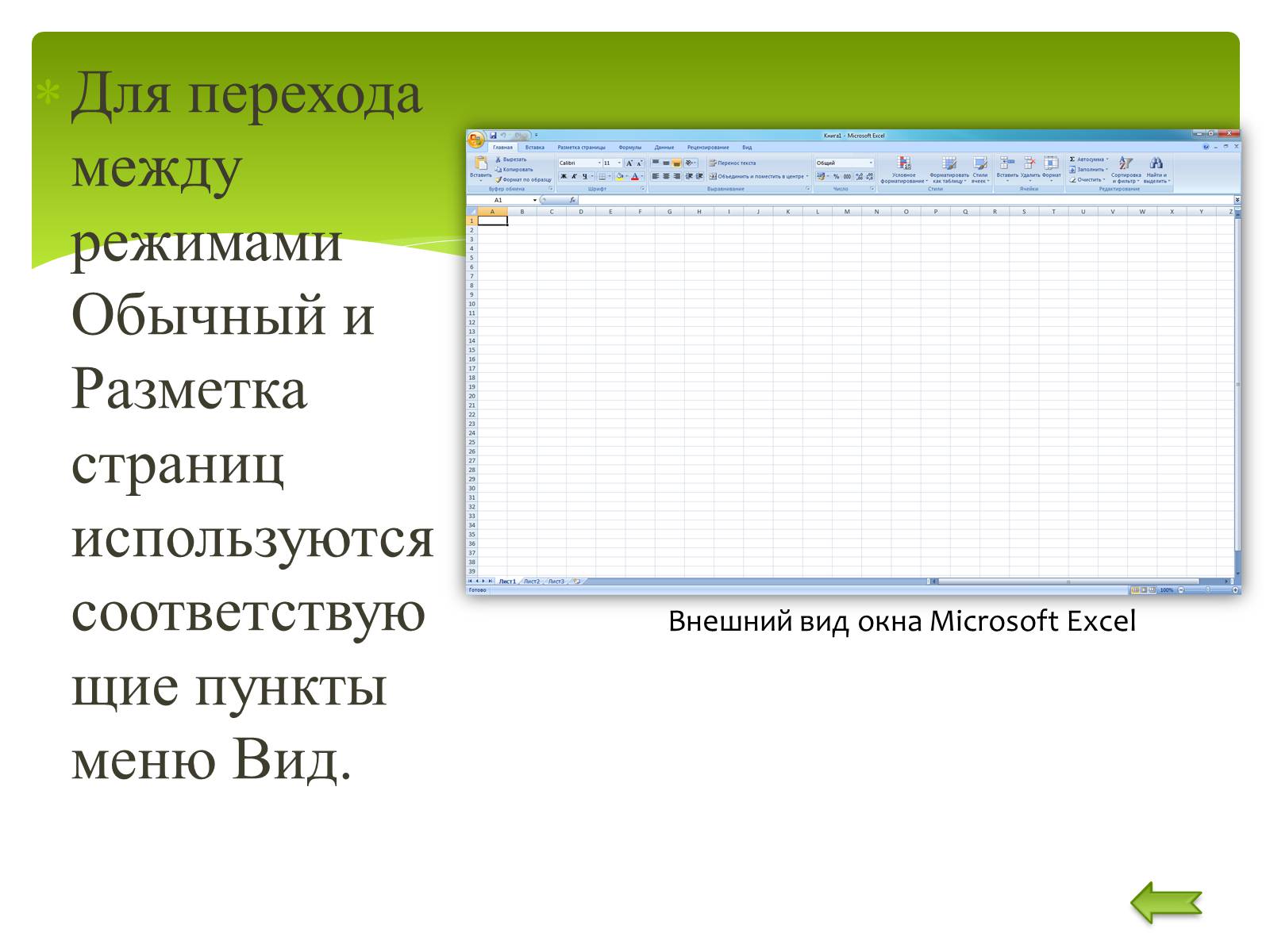
To switch between the Normal and Page Layout modes, use the corresponding items of the View menu.
Microsoft Excel window appearance
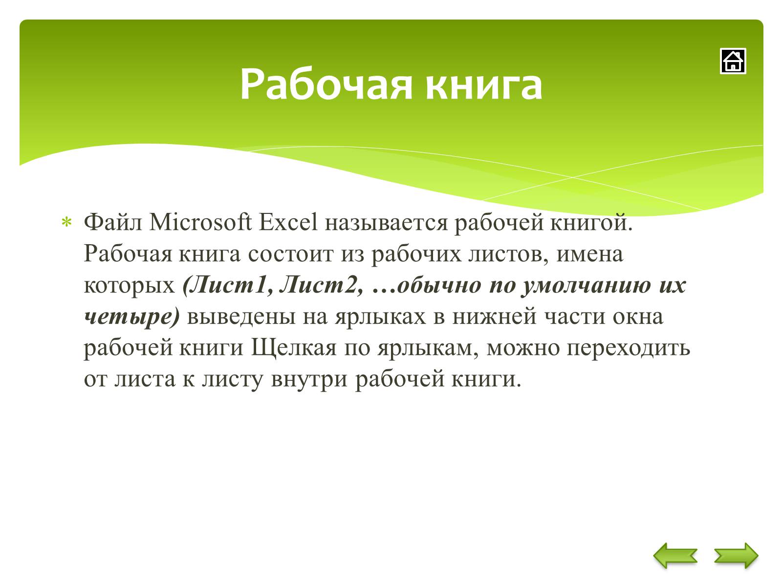
A Microsoft Excel file is called a workbook. A workbook consists of worksheets, the names of which (Sheet1, Sheet2, ... usually there are four by default) are displayed on the labels at the bottom of the workbook window. By clicking on the labels, you can move from sheet to sheet within the workbook.
Workbook

To create a new workbook, select the New command from the File menu. In the opened dialog box the template on the basis of which the workbook will be created; then click the OK button. Regular workbooks are created based on the Book template. You can click the button to create a workbook based on the Book template.
Creating a workbook
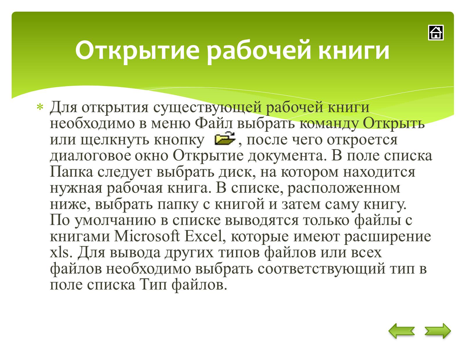
To open an existing workbook, select the Open command from the File menu, or click the button to open the Open Document dialog box. In the Folder list box, select the drive containing the required workbook. In the list below, select the folder with the workbook and then the workbook itself. By default, only files with Microsoft Excel workbooks that have the xls extension are displayed in the list. To display other types of files or all files, select the appropriate type in the File type list box.
Opening a workbook
Saving a workbook

Saving a workbook
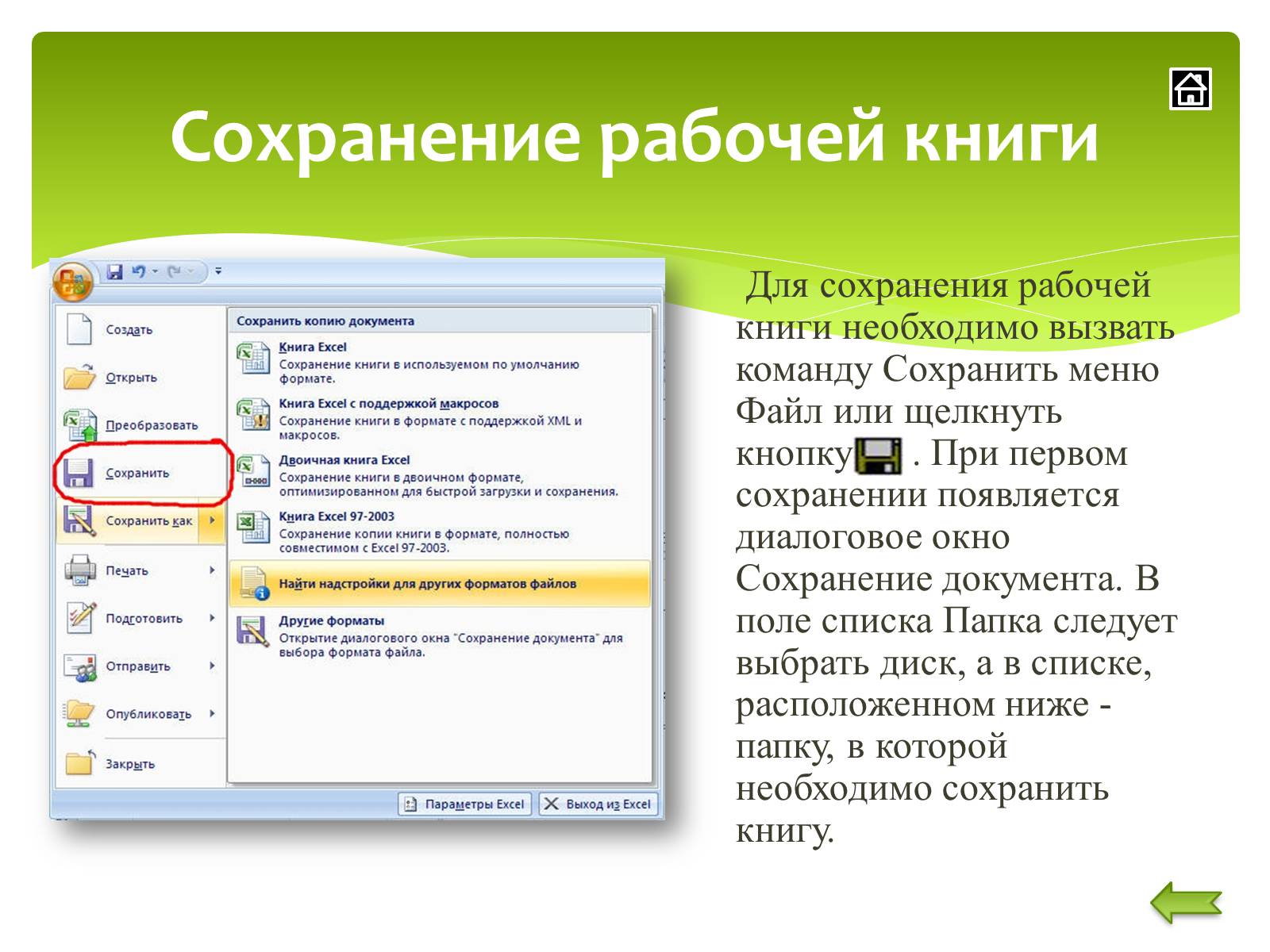
To save the workbook, call the Save command on the File menu or click the button. The first time you save, the Save Document dialog box appears. In the Folder list box, select the drive, and in the list below - the folder where you want to save the book.
Saving a workbook
To save the workbook, call the Save command on the File menu or click the button. The first time you save, the Save Document dialog box appears. In the Folder list box, select the drive, and in the list below - the folder where you want to save the book.

Worksheet
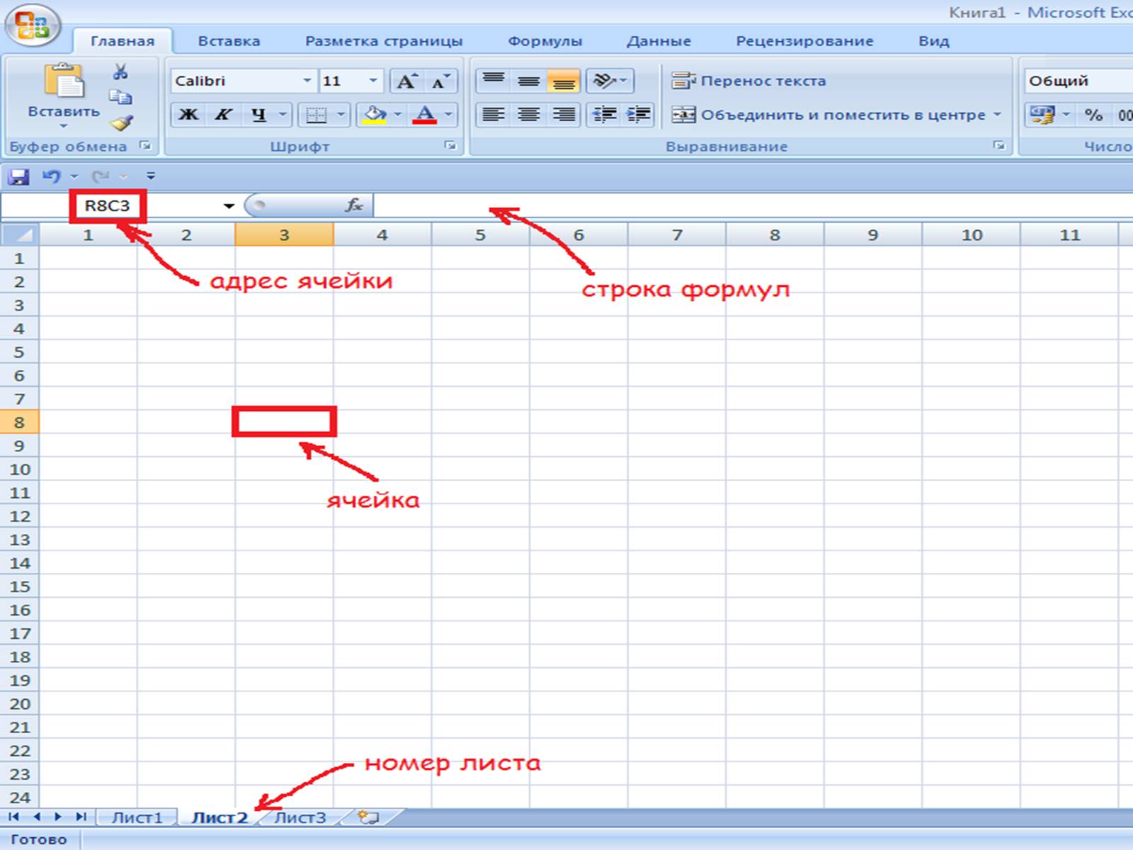
It is a table with 256 columns and 65536 rows. Columns are named in Latin letters, and rows are named in numbers. Each cell in a table has an address that consists of a row name and a column name. For example, if a cell is in column A and row 7, then it has the address A7. One of the table cells is always active. The active cell is highlighted with a frame. To make a cell active, you must use the cursor keys to move the frame to this cell or click in it with the mouse.

To select several adjacent cells, place the mouse pointer in one of the cells, press the left mouse button and, without releasing it, stretch the selection over the entire area. To select several non-adjacent groups of cells, select one group, press the Ctrl key and, without releasing it, select other cells. To select an entire column or table row, click on its name. To select multiple columns or rows, click on the name of the first column or row and stretch the selection to fill the entire area.
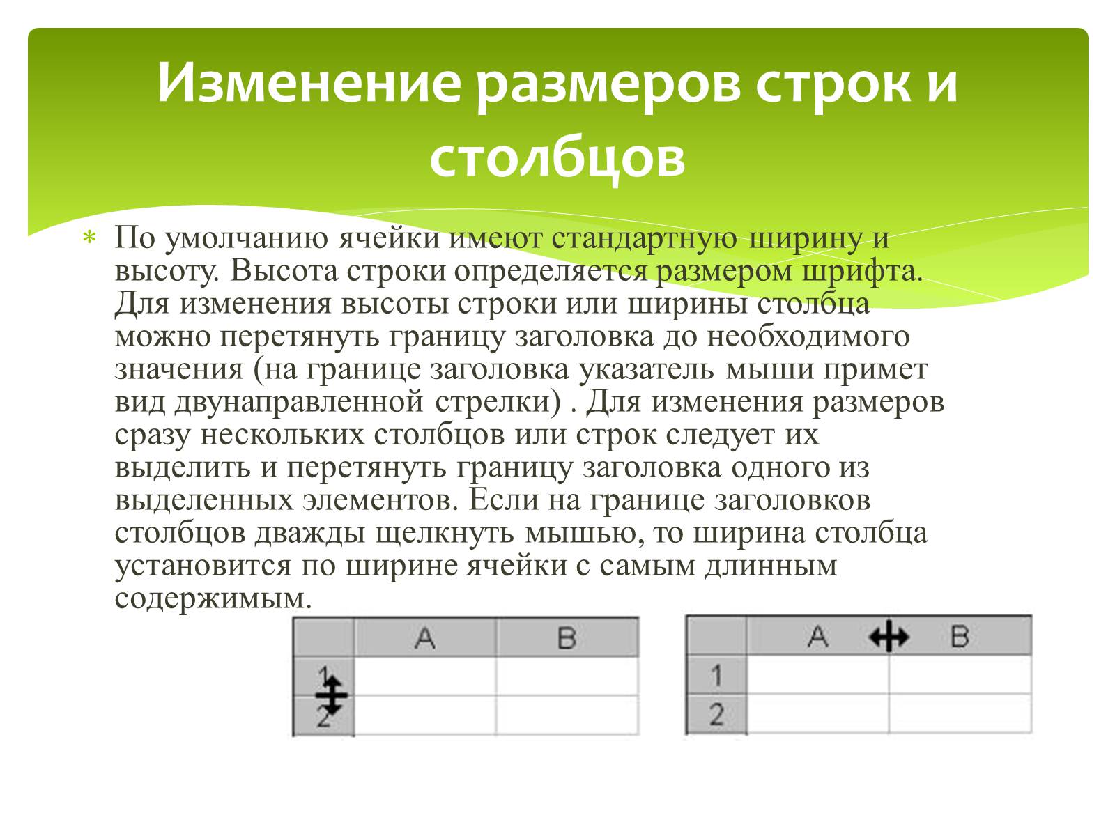
By default, cells have a standard width and height. The line height is determined by the font size. To change the row height or column width, you can drag the header border to the desired value (at the header border, the mouse pointer changes to a double-headed arrow). To resize several columns or rows at once, select them and drag the border of the header of one of the selected elements. If you double-click on the border of the column headings, the column width will be set to the width of the cell with the longest content.
Resizing rows and columns

Filling the cells
To enter data in a cell, you must make it active and enter data from the keyboard. The data will appear in the cell and in the edit line. To complete the entry, press Enter or one of the cursor keys.
To edit the contents of a cell, just double click on it.
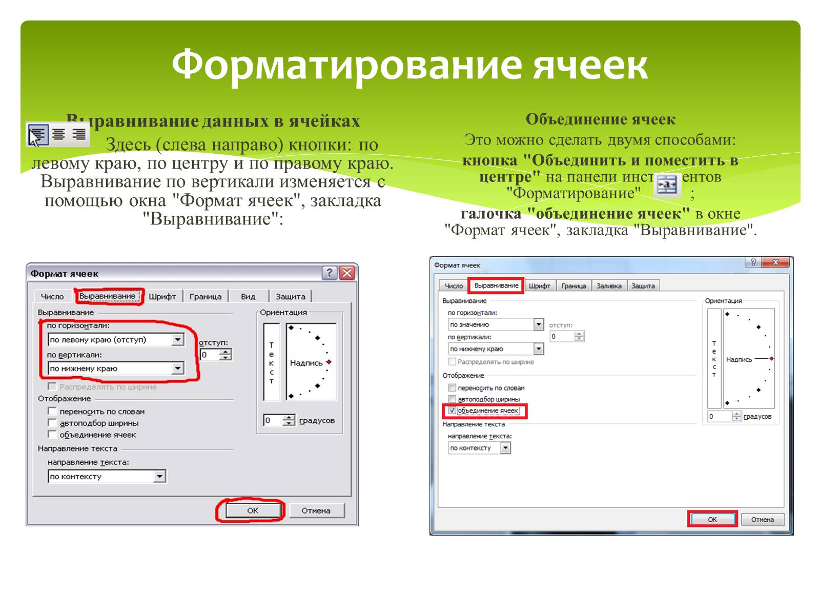
Formatting cells
Aligning data in cells
Here (from left to right) the buttons are: left-aligned, centered, and right-aligned. Vertical alignment is changed using the "Format Cells" window, the "Alignment" tab:
Merging cells
This can be done in two ways:
merge & Center button on the Formatting toolbar;
checkbox "merge cells" in the "Format cells" window, tab "Alignment".

Filling cells with color
There are two ways to change the fill color of the selected cells:
the "Fill Color" button on the "Formatting" toolbar;
"Format cells" window, "View" tab:
Adding cell borders
The default Excel sheet is a table. However, the table grid is not printed until we hover over them. There are three ways to add borders to selected cells:
"Borders" button on the "Formatting" toolbar;
window "Border", called from the button "Borders" -\u003e "Draw Borders ..."

By dragging the fill handle * of a cell, you can copy its data to other cells in the same row or the same column. If a cell contains a number, date, or time period, which can be part of a series, then its value is incremented when copied.
For example, if a cell has the value January, then you can quickly fill other cells in the row or column with February, March, and so on.
Custom autocomplete lists can be created for frequently used values, for example: a list of library performance indicators, names and positions of employees, a list of departments, etc.
Autocomplete based on adjacent cells

1. Specify the cell where you want to enter data.
2. Type data and press Enter.
When entering a date, use a period or hyphen as a separator, such as 05/09/99 or Jan-99.
Entering numbers, text, date or time of day:

1. Pick the first cell of the range to fill and enter a start value.
To specify an increment other than 1, select the second cell in the series and enter the corresponding value. The magnitude of the increment will be given by the difference in these values.
2. Select the cell or cells containing seed values.
3. Drag the fill handle over the cells to be filled.
To fill in ascending order, drag the handle down or to the right.
To fill in descending order, drag the handle up or left.
Filling in series of numbers, dates and other elements

1. Specify the cell where you want to enter the formula.
2. Enter \u003d (equal sign).
If you click Edit Formula or Insert Function, an equal sign is automatically inserted.
3. Enter the formula.
Formula diagram:
4. Press the Enter key.
Formula input:
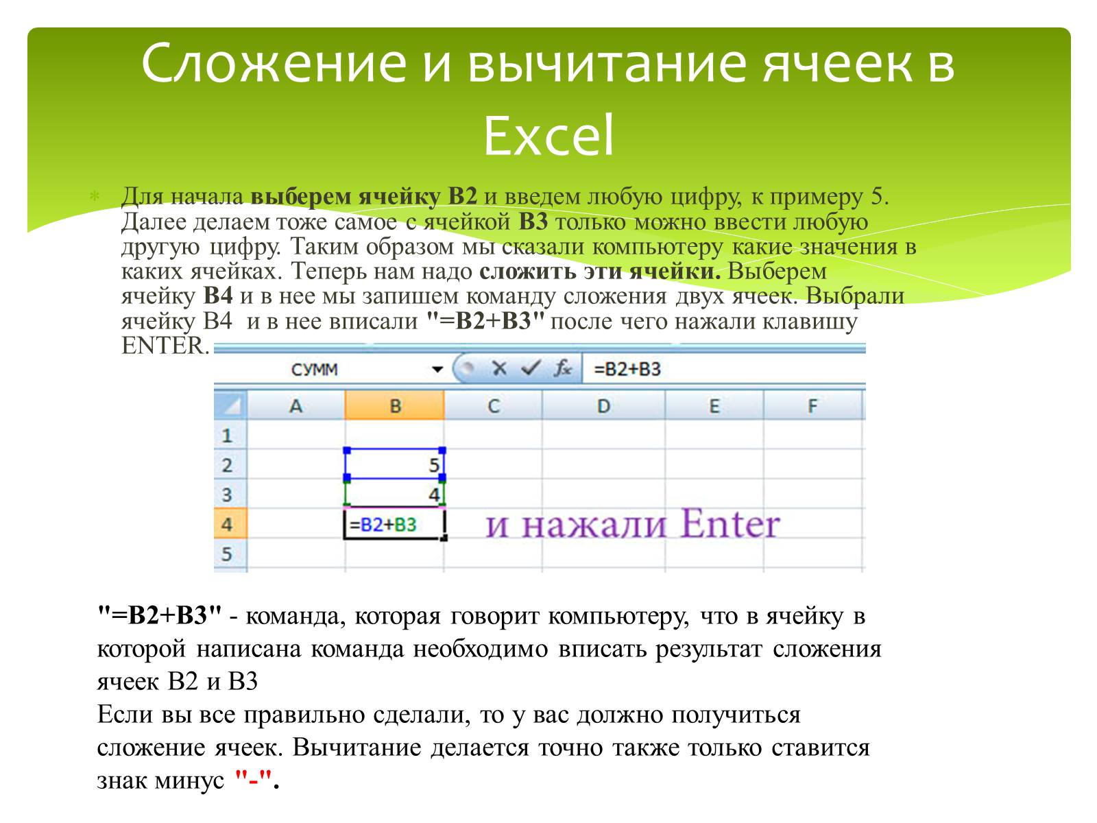
First, select cell B2 and enter any number, for example 5. Next, do the same with cell B3, only you can enter any other number. Thus, we told the computer which values \u200b\u200bare in which cells. Now we need to add these cells. Let's select cell B4 and in it we will write the command for adding two cells. We selected cell B4 and entered "\u003d B2 + B3" into it and then pressed the ENTER key.
Add and subtract cells in Excel
"\u003d B2 + B3" - a command that tells the computer that in the cell in which the command is written, the result of the addition of cells B2 and B3 must be entered
If you did everything correctly, then you should have a cell addition. Subtraction is done in the same way, only the minus sign "-" is put.

Calculations in tables are performed using formulas. A formula can consist of mathematical operators, values, cell references, and function names. The result of the formula execution is some new value contained in the cell where the formula is located. The formula starts with an equal sign "\u003d". The formula can use the arithmetic operators +, -, *, /. The order of calculations is determined by the usual mathematical laws. Examples of formulas: \u003d (D4 ^ 2 + B8) * A6, \u003d A7 * C4 + B2. etc.
Functions in Microsoft Excel are called combining several computational operations to solve a specific problem. Functions in Microsoft Excel are formulas that take one or more arguments. Numerical values \u200b\u200bor cell addresses are indicated as arguments, For example: \u003d SUM (A1: A9) - the sum of cells A1, A2, A3, A4, A5, A6, A7, A8, A9; To enter a function into a cell, you must: -select a cell for a formula; -call the Function Wizard using the Function command of the Insert menu or the button; -in the Function Wizard dialog box, select the function type in the Category field, then the function in the Function list; -click the OK button;
Basic types of actions

Header Row By default, a table includes a header line. Filtering is enabled for each column in the table in the header row, allowing you to quickly filter or sort data.
Elements of Microsoft Excel tables

Alternating lines
By default, the table uses a striped row background to improve the readability of the data.
Calculated columns
By entering a formula into one cell in a table column, you can create a calculated column that will immediately apply the formula to all other cells.

Totals line
You can add a totals row to a table that provides access to summarizing functions (for example, AVERAGE, COUNT, or SUM). Each cell in the totals row displays a drop-down list so you can quickly calculate the totals you want.
Resize handle
The resize handle in the lower-right corner of the table allows you to resize the table by dragging and dropping.

Related entries:
 Presentation on the topic "social structure and social relations" Social stratification by Weber
 The rapid development and expansion of the fields of application of electronic devices is due to the improvement of the element base, - presentation
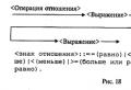 Boolean values, operations, expressions
 Von Neumann architecture presentation
 The history of the development of computer technology The beginning of the computer era


